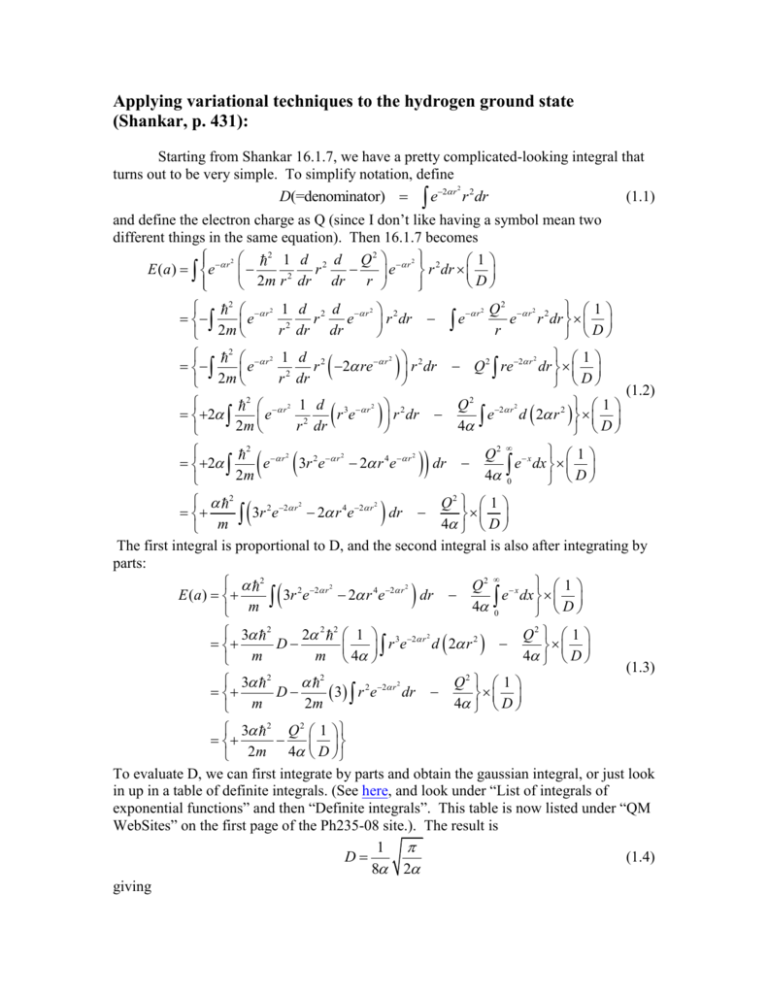
Applying variational techniques to the hydrogen ground state
(Shankar, p. 431):
Starting from Shankar 16.1.7, we have a pretty complicated-looking integral that
turns out to be very simple. To simplify notation, define
2
(1.1)
D(=denominator)   e2 r r 2 dr
and define the electron charge as Q (since I don’t like having a symbol mean two
different things in the same equation). Then 16.1.7 becomes
2
2 
1 d 2 d Q 2   r 2  2

1
E ( a )    e  r  
r

 e  r dr   
2
D
 2m r dr dr r 


2

  r 2 1 d 2 d  r 2  2
  
r
e
e
 r dr
r 2 dr dr

 2m 
2

  r 2 1
  
e
r2
 2m 
2

  r 2
 2 
e
2m 




 r
e
2
Q 2  r 2 2   1 
e r dr    
r
 D
2
 1
 Q 2  re 2 r dr    
 D
(1.2)

Q 2 2 r 2
1



e
d  2 r 2     
4 
 D
2
d 2

r 2 re  r  r 2 dr
dr



1 d 3  r 2  2
re
 r dr
r 2 dr

 
2

2
2
2
 2 
e  r 3r 2 e  r  2 r 4e  r
2m

 dr


Q2  x   1 
e dx    
4 0
 D
  2
Q2   1 
2 2 r 2
4 2 r 2
 
dr 
  
 3r e  2 r e
4   D 
 m
The first integral is proportional to D, and the second integral is also after integrating by
parts:

  2
Q2  x   1 
2 2 r 2
4 2 r 2
E (a)  
3
r
e

2

r
e
dr

e dx    

4 0
 m
 D




 3 2
2 2 2  1  3 2 r 2
Q2   1 
2
 
D
r
e
d
2

r



  


m  4  
4   D 
 m
 3 2
 2
Q2   1 
2 2 r 2
 
D
3
r
e
dr

 
  
2m
4   D 
 m
(1.3)
 3 2 Q 2  1  
 

 
 2m 4  D  
To evaluate D, we can first integrate by parts and obtain the gaussian integral, or just look
in up in a table of definite integrals. (See here, and look under “List of integrals of
exponential functions” and then “Definite integrals”. This table is now listed under “QM
WebSites” on the first page of the Ph235-08 site.). The result is
1 
(1.4)
D
8 2
giving
 3 2
2 
E (a)  
 2Q 2

 
 2m
Minimizing this as a function of  gives
(1.5)
2
 mQ 2  8
  a0   2 

 9
2
 Q2  8
mQ 4 8
1
8
 E (a0 )   2
   mc 2  
 E1
 0.849 Ry
 
2 3
2
3
 c  3
=========================================
Now let’s repeat the calculation, but using   e r as the trial wavefunction. Then
D(=denominator) 
e
2 r 2
(1.6)
(1.7)
r dr
and
2
  r 
1 d 2 d Q 2   r  2
1
E ( a )   e  
r

 e  r dr   
2
D


 2m r dr dr r 
2

 1
  r 1 d 2

  
r   e  r   r 2 dr  Q 2  re 2 r dr    
e
2
r dr

 2m 
 D
  2
 
 2m
  2re
2 r
(1.8)
 1
  r 2e 2 r  dr  Q 2  re 2 r dr    
 D
Now change variables to x  2 r , and we can do all the integrals in our head. We get
3
D  2  2 
(1.9)
and
3
  2  2
2 
Q 2    2  
E (a)  





2
3
2
 2 
2
m
2

2

2













 
2

Q 2 
 
2

1

 4 3 
 
2 
 2  
 8m
2

 2 2
Q2 
3
 
 2    4   
4 
 8m
 2m
Minimizing with respect to  gives
mQ 2
  2  a0
(=Bohr radius)
(1.10)

  Q2 

2
1 mQ 4
1
Q4
1
2
2  e 
E  a0   


mc


mc






2 2
2 2
2
c
2
 c
which are the expressions we know for the hydrogen ground state.
2
(1.11)