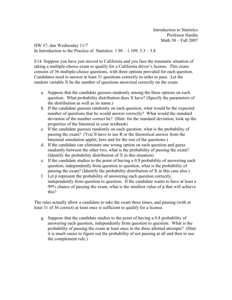
Introduction to Statistics
Professor Hardin
Math 58 – Fall 2007
HW #7, due Wednesday 11/7
In Introduction to the Practice of Statistics: 1.98 – 1.109, 5.3 – 5.8
E14. Suppose you have just moved to California and you face the traumatic situation of
taking a multiple-choice exam to qualify for a California driver’s license. This exam
consists of 36 multiple-choice questions, with three options provided for each question.
Candidates need to answer at least 31 questions correctly in order to pass. Let the
random variable X be the number of questions answered correctly on the exam.
a. Suppose that the candidate guesses randomly among the three options on each
question. What probability distribution does X have? (Specify the parameters of
the distribution as well as its name.)
b. If the candidate guesses randomly on each question, what would be the expected
number of questions that he would answer correctly? What would the standard
deviation of the number correct be? (Hint: for the standard deviation, look up the
properties of the binomial in your textbook)
c. If the candidate guesses randomly on each question, what is the probability of
passing the exam? (You’ll have to use R or the theoretical answer from the
binomial simulation applet, here and for the rest of the questions.)
d. If the candidate can eliminate one wrong option on each question and guess
randomly between the other two, what is the probability of passing the exam?
(Identify the probability distribution of X in this situation)
e. If the candidate studies to the point of having a 0.9 probability of answering each
question, independently from question to question, what is the probability of
passing the exam? (Identify the probability distribution of X in this case also.)
f. Let p represent the probability of answering each question correctly,
independently from question to question. If the candidate wants to have at least a
99% chance of passing the exam, what is the smallest value of p that will achieve
this?
The rules actually allow a candidate to take the exam three times, and passing (with at
least 31 of 36 correct) at least once is sufficient to qualify for a license.
g. Suppose that the candidate studies to the point of having a 0.8 probability of
answering each question, independently from question to question. What is the
probability of passing the exam at least once in the three allotted attempts? (Hint:
it is much easier to figure out the probability of not passing at all and then to use
the complement rule.)
E15. Birthweights of babies in the United States have been said to be reasonably modeled
by a normal distribution with mean 3250 grams and standard deviation 550 grams,
N(3250, 550). Babies weighing less than 2500 grams are considered to be of low
birthweight.
a. Produce a sketch of the normal density curve described by these parameters (with
appropriate scaling). Provide a label and a scale for the horizontal axis.
b. Approximately 68% of newborns weigh between which two values? Shade the
corresponding area of the distribution in (a).
c. On the graph in (a), shade the area of the distribution corresponding to babies of
low birthweight. Estimate from your shading the percentage of the distribution
that falls in this range.
d. To estimate the probability of a randomly selected baby being of low birthweight,
we will use the normal model to determine P(X ≤ 2500), where X, which denotes
the birthweight of a randomly selected baby, follows a N(3250, 550) distribution.
We can calculate the probabilities using R or an applet. The applet is slightly
more visual.
Open the “Normal Probability Calculator” applet and enter “birthweight” in the
variable box. Specify 3250 as the mean and 550 as the standard deviation. Press
the “Scale to Fit” button. Select the first row and in the X box, enter the value of
2500 and hit the Enter key. (Note the applet scales both the x-axis and the “zaxis”).
i. What does the applet report for the z-score and the probability?
ii. Write a one-sentence interpretation of the z-score and the above
probability.
e. Data from the National Vital Statistics Report indicate that there were 3,880,894
births in the United States in 1997. A total of 291,154 babies were of low
birthweight. What is the observed proportion of birthweight babies and how does
this compare to the proportion predicted by the normal model?
f. Suppose you wanted to estimate the probability of a baby weighing more than 10
pounds (4536 grams) at birth. Sketch (and label) the distribution and shade the
area of interest.
g. In the applet, change the inequality to >, specify 4536 in the “X” box, and press
Enter. What are the z-score and the probability reported by the applet? Confirm
that the numbers are consistent with your sketch.
h. Suppose you wanted to estimate the probability that a randomly selected baby
weights between 3000 and 4000 grams. Sketch (and label) the probability model
with the area of interest shaded.
i. In the applet, specify 3000 in the first “X” box, and then select the second row
and specify 4000 in the second “X” box. Press the Enter key. What does the
applet report for the z-scores and probability between these two values?
j. Data from the National Vital Statistics Report indicate that there were 2,552,852
newborns weighing between 3000 and 4000 grams in 1997. How closely does the
model’s prediction in (i) match the observed relative frequency?
k. You can also use the normal distribution model to “work backwards.” Suppose
you want to know how much a baby would have to weigh to be among the lightest
2.5% of all newborns (the 2.5th percentile). Sketch (and label) a normal model
and indicate the appropriate area on the sketch.
l. In the applet, unselect the second row. Since we want the lightest 2.5%, make
sure the first row inequality is set at < and change the “probability” box value ot
0.025. Hit the Enter key. The applet will determine the corresponding z-score
and weight. Are the results consistent with your sketch? Explain.
m. Use the applet to determine how much a baby would have to weigh at birth to be
in the heaviest 2.5% of all newborns. How does this z-score compare to that in (l)
and how do the weight cutoffs compare? Explain the relationships.
n. Suppose instead that birthweights of newborns followed a normal distribution
with mean 3500 and standard deviation 400. Use the applet to create this sketch
(pressing the “Scale to Fit” button) and to determine the two values such that the
middle 95% of birthweights fall in between the two values.
o. How do the z-scores in (n) compare to those in (l) and (m)?
p. Notice that R gives the same values as the applet. Use R to calculate the
probabilities in (d), (g), and (i). Write down the R commands you used.
q. You can also use R to calculate the percentile cutoffs. Recalculate the cutoffs
from (l), (m), and (n). Write down the R commands you used.