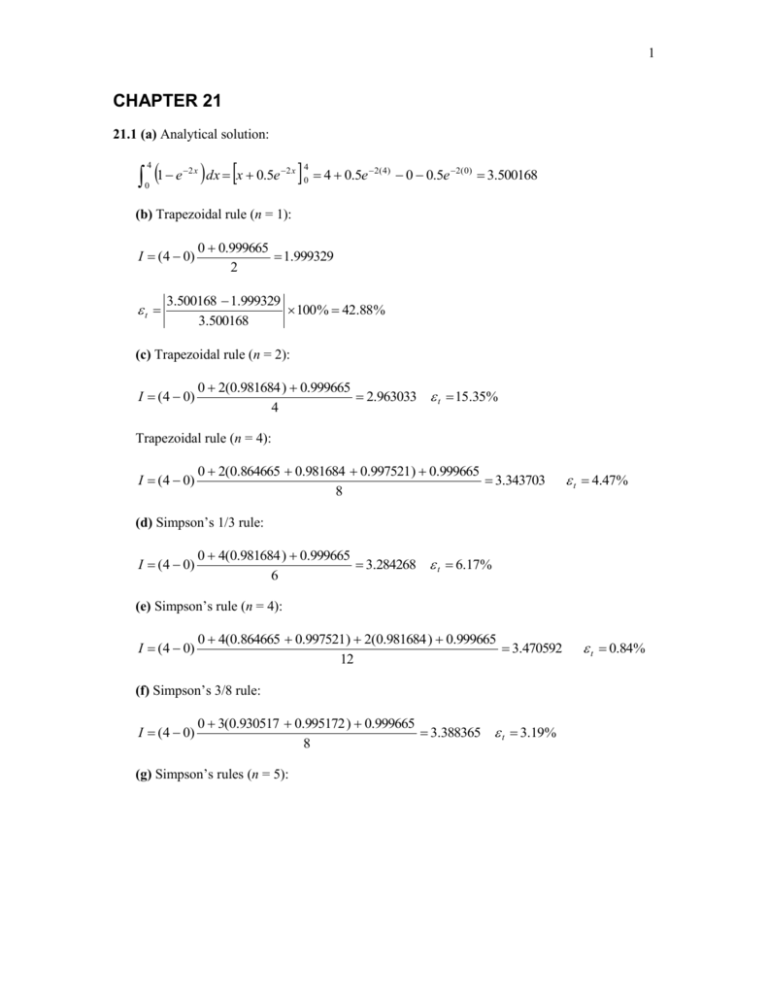
1
CHAPTER 21
21.1 (a) Analytical solution:
 1  e  dx  x  0.5e 
4
2 x
0
2 x 4
0
 4  0.5e 2( 4)  0  0.5e 2(0)  3.500168
(b) Trapezoidal rule (n = 1):
I  (4  0)
t 
0  0.999665
 1.999329
2
3.500168  1.999329
 100%  42.88%
3.500168
(c) Trapezoidal rule (n = 2):
I  (4  0)
0  2(0.981684 )  0.999665
 2.963033  t  15.35%
4
Trapezoidal rule (n = 4):
I  (4  0)
0  2(0.864665  0.981684  0.997521)  0.999665
 3.343703
8
 t  4.47%
(d) Simpson’s 1/3 rule:
I  (4  0)
0  4(0.981684 )  0.999665
 3.284268  t  6.17%
6
(e) Simpson’s rule (n = 4):
I  (4  0)
0  4(0.864665  0.997521)  2(0.981684 )  0.999665
 3.470592
12
(f) Simpson’s 3/8 rule:
I  (4  0)
0  3(0.930517  0.995172 )  0.999665
 3.388365  t  3.19%
8
(g) Simpson’s rules (n = 5):
 t  0.84%
2
I  (1.6  0)
0  4(0.798103 )  0.959238
6
 (4  1.6)
0.959238  3(0.99177  0.998338 )  0.999665
8
 1.107107  2.378769  3.485876
 t  0.41%
21.3 (a) Analytical solution:
4

4
2

x2
x6 
(1  x  4 x  2 x ) dx   x 
 x 4    1104
2
3  2

3
5
(b) Trapezoidal rule (n = 1):
I  (4  (2))
 29  1789
 5280
2
t 
1104  5280
 100%  378 .26%
1104
(c) Trapezoidal rule (n = 2):
I  (4  (2))
 29  2(2)  1789
 2634  t  138.59%
4
Trapezoidal rule (n = 4):
I  (4  (2))
 29  2(1.9375  2  131.3125 )  1789
 1516 .875
8
 t  37.398%
(d) Simpson’s 1/3 rule (n = 2):
I  (4  (2))
 29  4(2)  1789
 1752  t  58.7%
6
(e) Simpson’s 3/8 rule:
I  (4  (2))
 29  3(1  31)  1789
 1392  t  26.087%
8
(f) Boole’s rule (n = 5):
I  (4  (2))
7(29)  32(1.9375 )  12(2)  32(131.3125 )  7(1789 )
 1104
90
21.5 Analytical solution:
 t  0%
3

5
3
5
1

(4 x  3) dx   (4 x  3) 4   2056
16
 3
3
Simpson’s rule (n = 4):
I  (5  (3))
 3375  4(343  729)  2(1)  4913
 2056
12
 t  0%
Simpson’s rules (n = 5):
I  (0.2  (3))
 (5  0.2)
 3375  4(636 .056 )  10.648
6
 10.648  3(74.088  1191 .016 )  4913
 3162 .6  5218 .598  2056
8
 t  0%
Because Simpson’s rules are perfect for cubics, both versions yield the exact result for this
cubic polynomial.
21.7 Analytical solution:

1.5
0.5
1.5
14
2x
 1

dx  
14 2 x   517 .2301
 2 ln 14
 0.5
(a) Trapezoidal rule (n = 1):
I  (1.5  0.5)
14  2744
 1379
2
t 
517.2301  1379
 100%  166.612%
517.2301
(b) Simpson’s 1/3 rule (n = 2):
I  (1.5  0.5)
14  4(196)  2744
 590.3333  t  14.134%
6
(c) Simpson’s 3/8 rule:
I  (1.5  0.5)
14  3(81.323  472.3879 )  2744
 552.3916  t  6.798%
8
(d) Boole’s rule:
I  (1.5  0.5)
7(14)  32(52.3832 )  12(196)  32(733.3648 )  7(2744 )
 520.0215  t  0.5397 %
90
(e) Midpoint method:
I  (1.5  0.5)196  196
 t  62.106 %
4
(f) 3-segment-2-point open integration formula:
I  (1.5  0.5)
81.323  472.3879
 276.8554
2
 t  46.473%
(g) 4-segment-3-point open integration formula:
I  (1.5  0.5)
2(52.3832 )  196  2(733.3648 )
 458.4987
3
 t  11.355%
21.9 Analytical solution:
t
z (t ) 

t
0
m 
 gcd 
 gcd  
gm
tanh
t  dt   ln cosh
t  
 m 

 
cd
c
m




  0
 d 
10
 68.1 
 9.8(0.25)
 
z (10)  
ln cosh
(10)    333 .9262

 
68.1
 0.25 

  0
Thus, the result to 3 significant digits is 334. Here are results for various multiple-segment
trapezoidal rules:
n
1
2
3
4
5
6
7
8
9
10
11
12
13
14
I
246.9593
314.4026
325.4835
329.216
330.9225
331.8443
332.3984
332.7573
333.0031
333.1788
333.3087
333.4074
333.4842
333.5452
Thus, a 14-segment application gives the result to 4 significant digits.
21.11
(a) Trapezoidal rule (n = 6):
I  (10  (2))
35  2(5  10  2  5  3)  20
 65
12
5
(b) Simpson’s rules (n = 6):
I  (10  (2))
35  4(5  2  3)  2(10  5)  20
 56.66667
18
21.13 (a) Analytical solution:


0.6
2e 1.5 x dx   1.33333 e 1.5 x
0

0.6
0
 0.54209  (1.33333 )  0.79124
(b) Trapezoidal rule
I  (0.05  0)
2  1.8555
1.8555  1.597
1.597  1.3746
 (0.15  0.05)
 (0.25  0.15)
2
2
2
 (0.35  0.25)
1.3746  1.1831
1.1831  0.9808
 (0.475  0.35)
2
2
 (0.6  0.475)
t 
0.9808  0.8131
 0.79284
2
0.79124  0.79284
 100%  0.2022 %
0.79124
(c) Trapezoidal/Simpson’s rules
I  (0.05  0)
1.8555  3(1.597  1.3746 )  1.1831
2  1.8555
 (0.35  0.05)
2
8
 (0.6  0.35)
t 
1.1831  4(0.9808 )  0.8131
 0.791282
6
0.79124  0.791282
 100%  0.0052 %
0.79124
21.15 (a) Analytical solution:
2
2
1
2
0
3
  

2
( x  3 yz) dx dy dz 
 
2
3
2
0

 20  12 yz dy dz 
  40 z  12 z 2

2
2
2
 
2

 3 yzx
dy dz

0
4
 3
  20 y  6 y z
2
2
 160
(b) For z = –2, sweeping across the x dimension:
z = –2; y = 0:
1
2 x 4
2
2
0
dz 

2
2
 40  24 z dz
6
 27  4(1)  1
 20
6
I  (1  (3))
z = –2; y = 1:
 21  4(5)  7
4
6
I  (1  (3))
z = –2; y = 2:
I  (1  (3))
 15  4(11)  13
 28
6
These values can then be integrated along the y dimension:
I  (2  0)
 20  4(4)  28
8
6
For z = 0, similar calculations yield
z = 0; y = 0: I = –20
z = 0; y = 1: I = –20
z = 0; y = 2: I = –20
These values can then be integrated along the y dimension:
I  (2  0)
 20  4(20)  20
 40
6
For z = 2, similar calculations yield
z = 2; y = 0: I = –20
z = 2; y = 1: I = –44
z = 2; y = 2: I = –68
These values can then be integrated along the y dimension:
I  (2  0)
 20  4(44)  68
 88
6
Finally, these results can be integrated along the z dimension,
I  (2  (2))
8  4(40)  88
 160
6
 t  0%
21.17 Here is a VBA program that is set up to duplicate the computation performed in Example
21.5.
Option Explicit
Sub
Dim
Dim
Dim
TestSimpm()
n As Integer, i As Integer
a As Double, b As Double, h As Double
x(100) As Double, f(100) As Double
7
'Enter data and integration parameters
a = 0
b = 0.8
n = 4
h = (b - a) / n
'generate data from function
x(0) = a
f(0) = fx(a)
For i = 1 To n
x(i) = x(i - 1) + h
f(i) = fx(x(i))
Next i
'invoke function to determine and display integral
MsgBox "The integral is " & Simp13m(h, n, f)
End Sub
Function Simp13m(h, n, f)
Dim i As Integer
Dim sum As Double
sum = f(0)
For i = 1 To n - 2 Step 2
sum = sum + 4 * f(i) + 2 * f(i + 1)
Next i
sum = sum + 4 * f(n - 1) + f(n)
Simp13m = h * sum / 3
End Function
Function fx(x)
fx = 0.2 + 25 * x - 200 * x ^ 2 + 675 * x ^ 3 - 900 * x ^ 4 + 400 * x ^ 5
End Function
21.19 (a) Analytical solution:
M

11
0

5  0.25 x 2 dx  5x  0.083333 x 3

11
0
 165.9167
(b) Trapezoidal rule:
I  (1  0)
5  5.25
5.25  6
 (2  1)
     166.375
2
2
(c) Simpson’s rule:
I  (2  0)
5  4(5.25)  6
6  4(7.25)  9
 (4  2)
     165.9167
6
6
21.21 (a) Trapezoidal rule
I  (2  1)
56
6  5.5
m  min 60 s
 (3.25  2)
     60.375

 3,622.5 m
2
2
s
min
(b) Trapezoidal/Simpsons rules
8
I  (2  1)
6  4(5.5)  7
56
7  8.5
 (4.5  2)
 (6  4.5)
2
6
2
 (9  6)
8.5  3(8  6)  7
7  4(7)  5
m  min 60 s
 (10  9)
 59.9375

 3,596 .25 m
8
6
s
min
(c) We can use regression to fit a quadratic equation to the data
y = -0.1117x2 + 1.3526x + 3.4447
10
R2 = 0.5742
5
0
0
2
4
6
8
10
12
This equation can be integrated to yield
M


10
 0.1117 x 2 + 1.3526 x + 3.4447 dx   0.03723 x 3 + 0.6763 x 2 + 3.4447 x
1
 60.7599

10
1
m  min 60 s

 3,645 .594 m
s
min
We can use regression to fit a cubic equation to the data
y = -0.01646x3 + 0.16253x2 + 0.07881x + 4.85467
10
R2 = 0.63442
5
0
0
2
4
6
8
10
12
This equation can be integrated to yield
M

10
1
 0.01646 x 3 + 0.16253 x 2 + 0.07881x  4.85467 dx

  0.00412 x 4 + 0.054177 x 3 + 0.039405 x 2 + 4.85467 x
 60.56973

10
1
m  min 60 s

 3,634 .184 m
s
min
21.23 We can set up a table that contains the values comprising the integrand
t, hr
t, d
rate
(cars/4 min)
rate
(cars/d)
9
7:30
7:45
8:00
8:15
8:45
9:15
0.312500
0.322917
0.333333
0.343750
0.364583
0.385417
18
24
14
24
21
9
6480
8640
5040
8640
7560
3240
We can integrate this data using a combination of Simpson’s 3/8 and 1/3 rules. This yields the
number of cars that go through the intersection between 7:30 and 9:15,
I  (0.34375  0.3125 )
6480  3(8640  5040 )  8640
8
 (0.385417  0.34375 )
8640  4(7560 )  3240
6
 219.375  292.5  511.875 cars
The number of cars going through the intersection per minute can be computed as
511.875 cars hr
cars
 4.875
1.75 hr
60 min
min