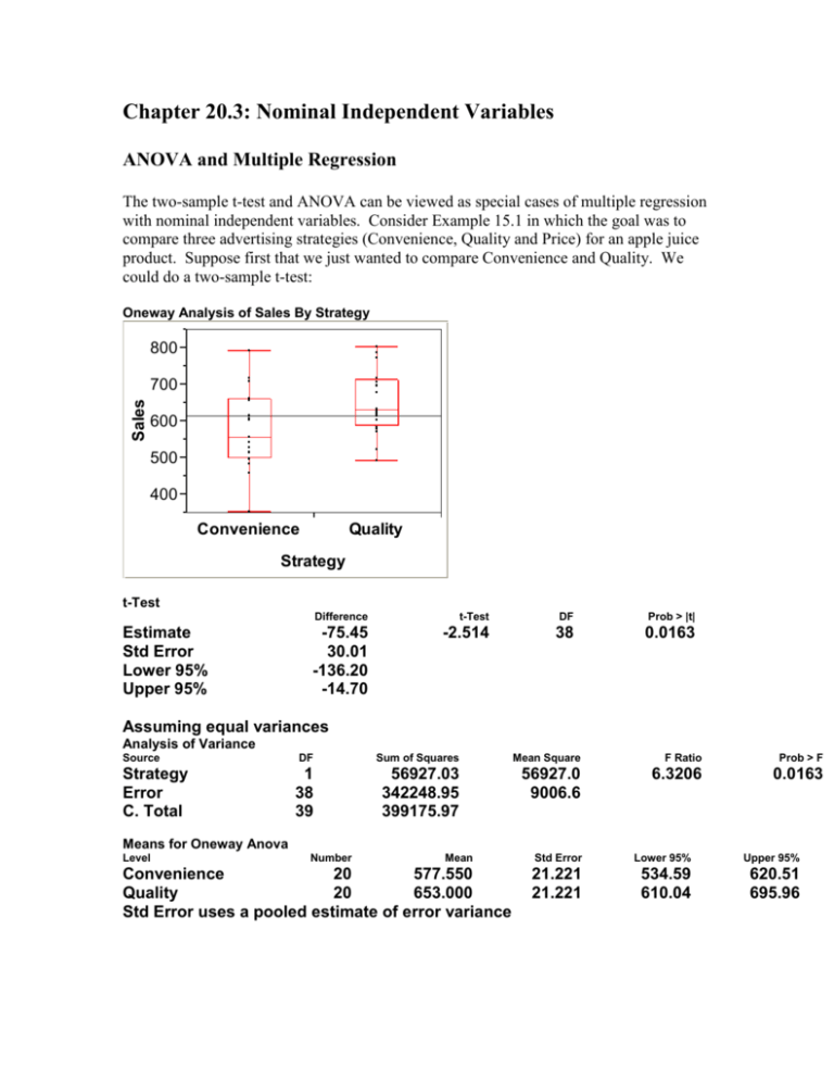
Chapter 20.3: Nominal Independent Variables
ANOVA and Multiple Regression
The two-sample t-test and ANOVA can be viewed as special cases of multiple regression
with nominal independent variables. Consider Example 15.1 in which the goal was to
compare three advertising strategies (Convenience, Quality and Price) for an apple juice
product. Suppose first that we just wanted to compare Convenience and Quality. We
could do a two-sample t-test:
Oneway Analysis of Sales By Strategy
800
Sales
700
600
500
400
Convenience
Quality
Strategy
t-Test
Estimate
Std Error
Lower 95%
Upper 95%
Difference
t-Test
DF
Prob > |t|
-75.45
30.01
-136.20
-14.70
-2.514
38
0.0163
Assuming equal variances
Analysis of Variance
Source
Strategy
Error
C. Total
DF
Sum of Squares
Mean Square
F Ratio
Prob > F
1
38
39
56927.03
342248.95
399175.97
56927.0
9006.6
6.3206
0.0163
Means for Oneway Anova
Level
Number
Mean
Convenience
20
577.550
Quality
20
653.000
Std Error uses a pooled estimate of error variance
Std Error
Lower 95%
Upper 95%
21.221
21.221
534.59
610.04
620.51
695.96
We could also consider a regression model. Let I1  0 if Convenience and I1  1 if
Quality. A regression model would look like this
Y   0  1 I 1 .
Bivariate Fit of Sales By I1
800
Sales
700
600
500
400
-0.2 0
.2
.4
.6
.8
1
1.2
I1
Linear Fit
Linear Fit
Sales = 577.55 + 75.45 I1
Summary of Fit
RSquare
RSquare Adj
Root Mean Square Error
Mean of Response
Observations (or Sum Wgts)
0.142611
0.120048
94.90285
615.275
40
Analysis of Variance
Source
Model
Error
C. Total
DF
Sum of Squares
Mean Square
F Ratio
1
38
39
56927.03
342248.95
399175.97
56927.0
9006.6
6.3206
Prob > F
0.0163
Parameter Estimates
Term
Intercept
I1
Estimate
Std Error
t Ratio
Prob>|t|
577.55
75.45
21.22092
30.01092
27.22
2.51
<.0001
0.0163
Notice that the coefficient on I1 equals the difference between the mean of quality (I1=1)
and the mean of convenience (I1=0). This makes sense because the coefficient on I1 is
the average change in sales for a one unit increase in I1. This just equals the difference
between the mean of quality and the mean of convenience. Also notice that the p-value
for testing whether I1=0 is the same as the p-value for the two-sided t-test.
What happens if we also want to incorporate the price strategy into the analysis, i.e., use a
one-way ANOVA with three levels for convenience, quality and price? The one-way
ANOVA analysis is the following:
Oneway Analysis of Sales By Strategy
800
Sales
700
600
500
400
Convenience Price
Each Pair
Student's t
0.05
Quality
Strategy
Oneway Anova
Summary of Fit
Rsquare
Adj Rsquare
Root Mean Square Error
Mean of Response
Observations (or Sum Wgts)
0.101882
0.07037
94.31038
613.0667
60
Analysis of Variance
Source
Strategy
Error
C. Total
DF
Sum of Squares
Mean Square
F Ratio
Prob > F
2
57
59
57512.23
506983.50
564495.73
28756.1
8894.4
3.2330
0.0468
Means for Oneway Anova
Level
Number
Mean
Convenience
20
577.550
Price
20
608.650
Quality
20
653.000
Std Error uses a pooled estimate of error variance
Means Comparisons
Dif=Mean[i]Mean[j]
Quality
Price
Convenienc
e
Quality
Price
Convenience
0.000
-44.350
-75.450
44.350
0.000
-31.100
75.450
31.100
0.000
Std Error
Lower 95%
Upper 95%
21.088
21.088
21.088
535.32
566.42
610.77
619.78
650.88
695.23
Alpha=
0.05
Comparisons for each pair using Student's t
t
2.00247
Abs(Dif)LSD
Quality
Price
Convenienc
e
Quality
Price
Convenience
-59.721
-15.371
15.729
-15.371
-59.721
-28.621
15.729
-28.621
-59.721
Positive values show pairs of means that are significantly different.
There is a multiple regression equivalent to the ANOVA but it involves creating two
dummy variables: I1  1 if quality, I1  0 if convenience or price and I 2  1 if price,
I 2  0 if convenience or quality. The regression model looks like this:
Y   0  1 I 1   2 I 2  
In this case the intercept  0 represents the mean for convenience,  0  1 represents the
mean for quality and  0   2 represents the mean for price.  1 represents the difference
between the means for quality and convenience and  2 represents the difference between
the means for price and convenience.
Response Sales
Whole Model
Actual by Predicted Plot
Sales Actual
800
700
600
500
400
400 500 600 700 800
Sales Predicted P=0.0468
RSq=0.10 RMSE=94.31
Summary of Fit
RSquare
0.101882
RSquare Adj
Root Mean Square Error
Mean of Response
Observations (or Sum Wgts)
0.07037
94.31038
613.0667
60
Analysis of Variance
Source
Model
Error
C. Total
DF
Sum of Squares
Mean Square
F Ratio
2
57
59
57512.23
506983.50
564495.73
28756.1
8894.4
3.2330
Prob > F
0.0468
Parameter Estimates
Term
Intercept
I1
I2
Estimate
Std Error
t Ratio
Prob>|t|
577.55
75.45
31.1
21.08844
29.82356
29.82356
27.39
2.53
1.04
<.0001
0.0142
0.3014
Effect Tests
Source
I1
I2
Nparm
DF
Sum of Squares
F Ratio
Prob > F
1
1
1
1
56927.025
9672.100
6.4003
1.0874
0.0142
0.3014
Sales Residual
Residual by Predicted Plot
200
100
0
-100
-200
400 500 600 700 800
Sales Predicted
Notice that the coefficients on I1 and I2 are the difference in sample means between
quality and convenience and between price and convenience respectively. Also notice
that the p-value for the F-test of H 0: 1   2  0 is identical to the p-value of the F-test
from one-way ANOVA of the hypothesis that the means of convenience, quality and
price are equal. This is the case because H 0: 1   2  0 is equivalent to the means of
convenience, quality and price being equal.
Combining Nominal Independent Variables and Continuous
Independent Variables
Multiple linear regression can accomodate both categorical independent variables and
continuous independent variables. For example (Keller and Warrack, section 20.3),
suppose you want to predict used-car prices from their odometer reading and their color
(white, silver and other). To represent the situation of three possible colors, we need two
indicator variables. In general to represent a nominal variable with m possible
categories, we must create m  1 indicator variables. Here, we create two indicator
variables.
I1  1 if the color is white
= 0 if the color is not white
I 2  1 if the color is silver
0 if the color is not silver
The category “Other colors” is defined by I1  0; I 2  0 .
Our regression model is
Y   0  1 X 1   2 I 1   3 I 2  
where X 1 equals odometer reading.
Response Price
Whole Model
Actual by Predicted Plot
Price Actual
16000
15500
15000
14500
14000
13500
13500 14500
15500
Price Predicted P<.0001
RSq=0.70 RMSE=284.54
Summary of Fit
RSquare
RSquare Adj
Root Mean Square Error
Mean of Response
Observations (or Sum Wgts)
0.69803
0.688594
284.5421
14822.82
100
Analysis of Variance
Source
Model
Error
C. Total
DF
Sum of Squares
Mean Square
F Ratio
3
96
99
17966997
7772564
25739561
5988999
80964
73.9709
Prob > F
<.0001
Parameter Estimates
Term
Intercept
Estimate
Std Error
t Ratio
Prob>|t|
16700.646
184.3331
90.60
<.0001
Term
Odometer
I-1
I-2
Estimate
Std Error
t Ratio
Prob>|t|
-0.05554
90.481959
295.47602
0.004737
68.16886
76.36998
-11.72
1.33
3.87
<.0001
0.1876
0.0002
Effect Tests
Source
Nparm
DF
Sum of Squares
F Ratio
Prob > F
1
1
1
1
1
1
11129137
142641
1211971
137.4575
1.7618
14.9692
<.0001
0.1876
0.0002
Odometer
I-1
I-2
Price Residual
Residual by Predicted Plot
800
600
400
200
0
-200
-400
-600
-800
13500
14500
15500
Price Predicted
The interpretation of the coefficient 90.48 on I1 is that a white car sells, on the average,
for $90.48 more than a car of the “Other Color” category with the same number of
odometer miles. The interpretation of the coefficient 295.48 on I2 is that a silver color
car sells, on the average for $295.48 more than a car of the “Other color” category with
the same number of odometer miles. The interpretation of the cofficient -.05554 on
odometer is that for two cars of the same color that differ in odometer by one, the car
with an additional mile on the odometer sells for 5.55 cents less on average.
For each color car, there is a regression line for how the average price depends on
odometer ( X 1 ). The regression lines for each color car are parallel. The indicator
variables can be interpreted as shifting the intercepts of the regression lines. See the
picture on page 708:
For white cars: Yˆ  (16700.65  90.48)  .056 X 1  16791.13  .056 X 1
For silver cars: Yˆ  (16700.65  295.48)  .056 X  16996.13  .056 X
1
1
For all other cars: Yˆ  16700.65  .056 X 1 .
Note: We will not consider it but it would be wise to investigate whether there was an
interaction between color and odometer. A more general multiple regression model
which would allow for different slopes and intercepts for each color of car would be
Y   0  1 X 1   2 I 1   3 I 2   4 X 1 * I 1   5 X 1 * I 2   .
Example: Problem 20.23
The president of a company that manufactures car seats has been concerned about the
number and cost of machine breakdowns. The problem is that the machines are old and
becoming quite unreliable. However, the cost of replacing them is quite high, and the
president is not certain that the cost can be made up in today’s slow economy.
In Exercise 18.85, a simple linear regression model was used to analyze the relationship
between welding machine breakdowns and the age of the machine. The analysis proved
to be so useful to company management that they decided to expand the model to include
other machines. Data were gathered for two other machines. These data as well as the
original data are stored in file Xr20-23 in the following way:
Column 1: Cost of repairs
Column 2: Age of machine
Column 3: Machine (1= welding machine; 2= lathe; 3=stamping machine)
(a) Develop a multiple regression model
(b) Interpret the coefficients
(c) Can we conclude that welding machines cost more to repair than stamping machines
if the machines are of the same age?
Solution:
(a) Y=Cost of repairs. We want to include as independent variables both the continuous
variable Age of Machine ( X 1 ) and the nominal variable Machine. To include the
nominal variable, we need to create two indicator variables (because the nominal variable
takes on three values). Let
I1  1 if the machine is a welding machine
= 0 if the machine is not a welding machine
I 2  1 if the machine is a lathe
0 if the machine is not a lathe
Our multiple regression model is
Y   0  1 X 1   2 I 1   3 I 2  
Response Repairs
Whole Model
Actual by Predicted Plot
Repairs Actual
500
400
300
200
100
100 200 300 400 500
Repairs Predicted P<.0001
RSq=0.59 RMSE=48.591
Summary of Fit
RSquare
RSquare Adj
Root Mean Square Error
Mean of Response
Observations (or Sum Wgts)
0.593778
0.572016
48.59141
340.6457
60
Analysis of Variance
Source
Model
Error
C. Total
DF
Sum of Squares
Mean Square
F Ratio
3
56
59
193271.36
132223.03
325494.39
64423.8
2361.1
27.2852
Prob > F
<.0001
Parameter Estimates
Term
Intercept
Age
I-1
I-2
Estimate
Std Error
t Ratio
Prob>|t|
119.25213
2.538233
-11.75534
-199.3737
35.00037
0.402311
19.70184
30.71301
3.41
6.31
-0.60
-6.49
0.0012
<.0001
0.5531
<.0001
Effect Tests
Source
Age
I-1
I-2
Nparm
DF
Sum of Squares
F Ratio
Prob > F
1
1
1
1
1
1
93984.714
840.574
99497.022
39.8050
0.3560
42.1397
<.0001
0.5531
<.0001
Residual by Predicted Plot
Repairs Residual
150
100
50
0
-50
-100
100 200 300 400 500
Repairs Predicted
The residual by predicted plot does not show any gross departures from a random scatter.
(b) For each additional month of age, repair costs increase on average by $2.54 for
machines of the same type; welding machines cost on average $11.76 less to repair than
stamping machines for the same age of machine; lathes cost on average $199.40 less to
repair than stamping machines for the same age of machine.
(c) To test whether welding machines cost more on average to repair than stamping
machines if the machines are of the same age, we want to test whether the coefficient on
I-1 is zero, i.e., we want to test H 0 :  2  0 . The p-value for the two-sided test is 0.5531.
Thus, there is not enough evidence to conclude that welding machines cost more on
average to repair than stamping machines if the machines are of the same age.
Practice Problems from Chapter 20: 20.6, 20.8, 20.20, 20.24