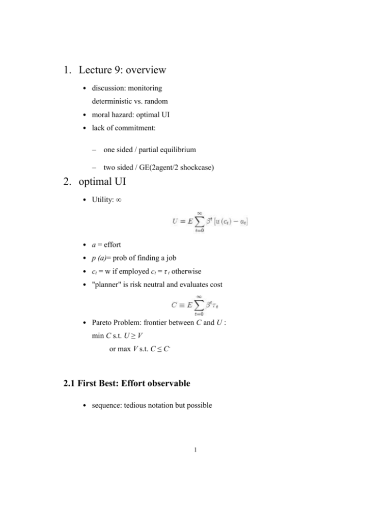
1. Lecture 9: overview
․ discussion: monitoring
deterministic vs. random
․ moral hazard: optimal UI
․ lack of commitment:
–
one sided / partial equilibrium
–
two sided / GE(2agent/2 shockcase)
2. optimal UI
․ Utility: ∞
․ a = effort
․ p (a)= prob of finding a job
․ ct = w if employed ct = τ t otherwise
․ "planner" is risk neutral and evaluates cost
․ Pareto Problem: frontier between C and U :
min C s.t. U ≥ V
or max V s.t. C ≤ C-
2.1 First Best: Effort observable
․ sequence: tedious notation but possible
1
․ recursive:
C (V )= min {c + β (1 − p (a)) C (V u)}
V = u (c) − a + β (1 − p (a)) V u + βp (a) V e
․ focs:
1−θ=0
β (1 − p (a)) C’(V u) − θβ (1 − p (a)) = 0
−βp’(a) C (V u)+ θβp’(a) V u − θβp’(a) V e + θ = 0
․ simplifying
․ result: Vtu is constant → ctu is constant
2.2 Second Best: Effort Unobservable
․ sequence problem is not very tractable (Shavell and Weiss perform a
variational argument for their results)
․ recursive formulation
C (V ) = min {c + β (1 − p (a)) C (V u)}
V = u (c) − a + β (1 − p (a)) V u + βp (a) V e
Βp’ (a)[V e − V u] = 1
․ focs
2
․ simplifying:
envelope condition implies
’
C (V ) = θ
․ results:
Vtu is decreasing
→ (using envelope and f.o.c. w.r.t. c) cut decreasing
Remarks:
․ relaxing cet = w (Hopenhayn and Nicolini, 1997)
․ agents save / borrow
․ welfare gains of optimal program
3. Lack of commitment: One Sided / Partial
Equilibrium
Source: LS Chapter 15 section 401-409
3
foc
‘
(λs + μπs) u (cs)= πs
’
λs + μπs = −πsP (ws)
combing:
since P is decreasing and concave then cs is increasing in ws.
․ ws = w if constraint not binding μ =0
․ otherwise ws > w
․ dynamics:
eventually converge to a high enough w so that participation constraint
is not binding (this result is more general: see Debraj Ray’s Econometrica paper)
4. Two Sided / GE
Sources:
․ LS Chapter 15 section 413-418: good treatment of Kocherlakota (iid shocks)
but no formal analysis of long-run distribution
․ we follow: simplified version of Alvarez-Jermann (2000) “Quantitative
Asset Pricing Implications of Endogenous Solvency Constraints”. only
section 4 and sub-section 5.1 (section 3 introduces the notation).
This version has individual persistence of income (not necessarily iid),
only 2 shocks, no aggregate shocks (in our version). We are able to
study the whole dynamics.
4.1 Dynamics
․ environment:
–
symmetric, two agents i =1, 2; equal population
4
–
y1 > y2,yt = y1 + y2 ≡ e (no aggregate uncertainty)
–
aggregate state s =1, 2 denotes realization of income for type 1
(equivalently: s denotes who gets high shock)
–
p is probability of transition from s =1 to s = 2 and from s = 2
to s’ = 1
․ Problem (recursive version)
․ last two constraints equivalent to
’
’
for some L (s ) and H (s )
․ we take as given that we have V, L and H
properties: V is decreasing, differentiable and concave in w
we then derive some properties of the allocation
․ graphical analysis: two shock case
․ first order conditions:
5
․ Envelope condition:
V1 (w,s) = −θ
․ result 1 : c (w,s) is increasing in w
2
since V is concave V1 is decreasing thus −V1 is increasing in w:
which requires c2 to increase with w
․ result 2 : if s = s’ then w (s’)= w. FOC:
is satisfied with equality if (w’ (s’) ,s’) = (w,s) . This satisfies the con- straint
since w ∋ [L (s) ,H (s)] by assumption.
․ result 3 : in the 2 shock case if s ≠ s’
․ collecting results:
–
–
–
–
–
c2 (w,s) is increasing in w
if s’ = s → w’ (s’) = w (constraint not binding)
if s ≠ s’ if binding then go to closest value possible
show graph of policy
convergence (main result): stationary distribution is history
independent and symmetric (we turn to studying this in more
detail next)
4.2 Stationary Distributions
Given our previous result we now look for stationary symmetric distributions:
․ given (c1,c2) let V 1 (c1,c2) and V 2 (c1,c2) be the unique solutions to:
Clearly: V2(y,x) = V1(x,y)
6
․ grinding out:
․ stationary symmetric feasible allocations satisfies:
i.e. resource constraint and participation constraints.
․ substituting
rearranging
if c1 ≤ y1 then (4) implies (5)  participation constraint for type 2
never binds
․ full risk sharing is attainable iff
․ otherwise, look for allocations with:
and y2 ≤ c2 ≤ c1≤ y1 (i.e. with less variability than autarky).
7
․ example: u (c)= c1−σ / (1 − σ) then
․ gives us c (ω) is decreasing in ω :
and we have ω (β,p) (increasing in β and p)
․ implications risk sharing
– decreasing in p
– decreasing in β
– increasing in risk aversion
5. Trash
5.1 Grinding V i (·, ·) formula
From
we get that
so (1 − β) V is a weighted average of u (c ) and u (c ).
2
1
8
2