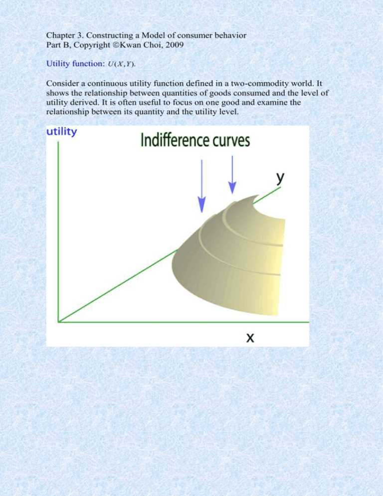
Chapter 3. Constructing a Model of consumer behavior
Part B, Copyright Kwan Choi, 2009
Utility function: U ( X , Y ).
Consider a continuous utility function defined in a two-commodity world. It
shows the relationship between quantities of goods consumed and the level of
utility derived. It is often useful to focus on one good and examine the
relationship between its quantity and the utility level.
Utility Curve
It shows the relationship between one good and the utility level, holding the
quantities of all other goods consumed.
2
Marginal utility of a good X is the increment of utility attributable to an extra
unit of X. In Figure 5, it is
MU X 
U
.
X
Indifference Curve
A locus of consumption bundles along which the utility level remains the
same.
3
Characteristics of Indifference Curves
1. Indifference curves are negatively sloped.
It follows from the nonsatiation assumption.
2.
Indifference curves are nonintersecting.
It follows from Transitivity and nonsatiation.
If two indifference curves, I and II, intersect one another, then a I b and c I a
imply c I b. However, bundle b dominates c, and hence bundle b is strictly
4
preferred to c, and b P c. This is a contradiction. Thus, indifference curves
cannot intersect one another.
3.
A higher indifference curve represents a higher utility level.
It follows from nonsatiation.
4.
Indifference curves are convex to the origin.
This follows from convexity of preferences.
Example: Consider a utility function U  XY . If the individual consumer
chooses ( X , Y )  (4, 6), then
U (4, 6)  24.
Similarly, if ( X , Y )  (6, 4), then
U (6, 4)  24.
Thus, both points (4,6) and (6,4) are on the same indifference curve. The
average of the two bundles is ( X , Y )  (5,5). And the utility of the average bundle
is:
U (5,5)  25.
Thus, the average bundle yields a higher utility. This utility function yields
convex indifference curves.
Marginal Rate of Substitution (MRS of x1 for x2) = is the amount of x2 that
the consumer is willing to give up to get an additional unit of x 1 to maintain the
same level of utility.
MRS  
5
X 2
.
X 1
6
Principle of Diminishing MRS: It follows from the convexity of preferences.
7
In Figure 9, marginal utility of x1 is zero. Marginal utility of good 2 is positive
if U > U' > U".
Straight-line indifference curves: Goods are perfect substitutes.
Flat indifference curves: marginal utility of one good is zero in some range.
8
The slope of indifference curves shows the rate of substitution.
Right angle indifference curves: goods are perfect complements.
9
10
Bowed-out indifference curves: Nonconvex preferences.
11
Fat indifference curves: Monotonicity is violated
Indifference curves are supposed to have no thickness, like a hypothetical, thin
pancake with only one side (I have not see one yet).
We cannot physically draw such indifference curves due to technical difficulty.
But if an individual really has a fat indifference curve, he would not be rational.
In Figure 13, bundle a has more of both goods than bundle b. Thus, a must be
preferred to b. Thus, those two points cannot be on the same indifference curve.
Marginal Utility (again)
Since there are many consumption goods, it is necessary to distinguish marginal
utilities of different goods. For instance, marginal utility of good 1 is the
increment of utility attained from an extra unit of that good, and is written as:
12
MU1 
13
U
.
X 1
Note that units of measurement are arbitrary. Hence, marginal utilities of the
same good can differ if the extra units are measured in gram or kilogram or
pound. It is often useful to measure marginal utilities when the extra unit
becomes extremely small, or infinitesimally small.
In Figure 14, marginal utility is the slope of the line AB. However, as ΔX
becomes infinitesimally small or approaches zero, line AB approaches the
tangent line AD. For practical reasons, it is safe to argue that marginal utility is
the slope of the tangent line AD (at the consumption point A).
Marginal utilities are measured while all other goods are held constant. Thus,
marginal utility of X is a partial derivative of U with respect to X.
MU X 
dU
U U
 lim

.

x

dX
X X
Example:
Let
U ( X , Y )  XY
be the utility function.
Derive marginal utilities of X and Y when evaluated at X = 5, and Y = 7.
MU X 
U
 Y  7,
X
(1)
MU Y 
U
 X  5.
Y
(2)
Derive the marginal utilities of X and Y when U ( X , Y )  X 1/ 3Y 2/ 3.
2
1 2 2 1  Y 3
MU X  X 3Y 3    .
3
3 X 
(3)
1
2 13  13 2  X  3
MUY  X Y    .
3
3 Y 
14
(4)
Marginal Rate of Substitution (again)
Along a given indifference curve, consumption of two goods can be changed
without altering the utility level. This means that on an indifference curve,
dU 
U
U
dx1 
dx2  MU1dx1  MU 2 dx2  0,
x1
x2
The slope of the indifference curve is the ratio of marginal utilities:

dx2 MU1

.
dx1 MU 2
In Figure 15, marginal rate of substitution (of x 1 for x2) is the slope of the ray
AB. However, here the change in good 1 (Δx1) is rather large. As Δx1 becomes
infinitesimally small or approaches zero, the slope of line AB approaches the
tangent line AD. Thus, for practical reasons, it is safe to say that MRS at point
A is the slope of the indifference curve (at that point).
Budget Constraint
Let M be the amount of money income to be spent on consumption goods. Then
the budget constraint is written as:
M  p1 X1  p2 X 2 ,
15
where p1 and p2 are prices of goods 1 and 2, respectively.
In Figure 15, AB is the budget line. The equation for the budget line is:
X2 
M p1

X 1.
p2 p2
Remember here the slope of the budget line is p1 / p2 —if the minus sign is
ignored— which is the relative price of the two goods.
Effect of a Price Increase
An increase in the price of good 1 rotates the budget line counterclockwise.
16
Increase in Income
An increase in income causes an outward, parallel shift in the budget line.
17
Constrained Optimization
The consumer chooses a consumption point along the budget line so as to
maximize his utility. This means a tangency point between the highest
indifference curve and the budget line.
18
At point B, the two curves are tangent each other, i.e.,
(the slope of the indifference curve) MRS 
p1
(the slope of the budget line)
p2
Why consumers do not buy a certain commodity
They may choose a corner solution.
19
20
Concave Indifference Curves
Always a corner solution occurs.
21