The Normal Distribution
The normal, or Gaussian, distribution has played a prominent role in statistics. It was
originally investigated by persons interested in gambling (Abraham de Moivre, 1733) or in the
distribution of errors made by persons observing astronomical events (Pierre-Simon Laplace, 1783
and Carl Friedrich Gauss, 1809). Adolphe Quetelet, also a philosopher and an astronomer, was a
pioneer in extending application of the normal curve to the social sciences.
The normal curve is still very important to behavioral statisticians because:
1. Many variables are distributed approximately as the bell-shaped normal curve.
2. Many of the inferential procedures (the so-called “parametric” tests) we shall learn assume that
variables are normally distributed.
3. Even when a variable is not normally distributed, a distribution of sample sums or means on that
variable will be approximately normally distributed if sample size is large.
4. Most of the special probability distributions we shall study approach a normal distribution under
some conditions.
5. The mathematics of the normal curve are well known and relatively simple. One can find the
probability that a score randomly sampled from a normal distribution will fall within the interval a to
b by integrating the normal probability density function (pdf) from a to b. This is equivalent to
finding the area under the curve between a and b, assuming a total area of one.
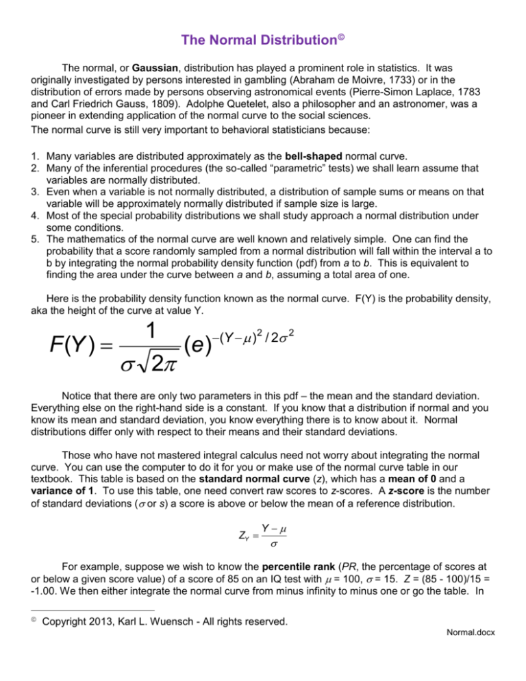
Here is the probability density function known as the normal curve. F(Y) is the probability density,
aka the height of the curve at value Y.
1
(Y   )2 / 2 2
F (Y ) 
(e)
 2
Notice that there are only two parameters in this pdf – the mean and the standard deviation.
Everything else on the right-hand side is a constant. If you know that a distribution if normal and you
know its mean and standard deviation, you know everything there is to know about it. Normal
distributions differ only with respect to their means and their standard deviations.
Those who have not mastered integral calculus need not worry about integrating the normal
curve. You can use the computer to do it for you or make use of the normal curve table in our
textbook. This table is based on the standard normal curve (z), which has a mean of 0 and a
variance of 1. To use this table, one need convert raw scores to z-scores. A z-score is the number
of standard deviations ( or s) a score is above or below the mean of a reference distribution.
ZY 
Y 

For example, suppose we wish to know the percentile rank (PR, the percentage of scores at
or below a given score value) of a score of 85 on an IQ test with  = 100,  = 15. Z = (85 - 100)/15 =
-1.00. We then either integrate the normal curve from minus infinity to minus one or go the table. In

Copyright 2013, Karl L. Wuensch - All rights reserved.
Normal.docx
~2~
the normal curve table in your text, find the row with Z = 1.00 (ignore the minus sign for now). Draw a
curve, locate the mean and -1.00 on the curve and shade the area you want (the lower tail). The entry
under “Smaller Portion” is the answer, .1587 or 15.87%.
Suppose IQ = 115, Z = +1.00. Now the answer is under “Larger Portion,” 84.13%.
What percentage of persons have IQ’s between 85 and 130? The Z-scores are -1.00 and
+2.00. Between the -1.00 and the mean are 34.13%, with another 47.72 between the mean and
+2.00, for a total of 81.85%.
What percentage have IQ’s between 115 and 130 ? The Z-scores are +1.00 and +2.00.
97.72% are below +2.00, 84.13% are below +1.00, so the answer is 97.72 - 84.13 = 13.59%.
What score marks off the lower 10% of IQ scores ? Now we look in the “Smaller Portion”
column to find .1000 . The closest we can get is .1003 , which has Z = 1.28 . We could do a linear
interpolation between 1.28 and 1.29 to be more precise. Since we are below the mean, Z = -1.28 .
What IQ has a Z of -1.28 ? X =  + Z ,
IQ = 100 + (-1.28) (15) = 100 - 19.2 = 80.8 .
What scores mark off the middle 50% of IQ scores? There will be 25% between the mean and
each Z-score,so we look for .2500 . The closest Z is .67, so the middle 50% is between Z = -0.67 and
Z = +0.67, which is IQ = 100 - (.67)(15) to 100 + (.67)(15) = 90 through 110.
You should memorize the following important Z-scores:
This Middle Percentage of Scores
50
68
90
95
98
99
100
Fall Between Plus and Minus z =
.67
1.
1.645
1.96
2.33
2.58
3.
There are standard score systems (where raw scores are transformed to have a preset mean
and standard deviation) other than z For example, SAT scores and GRE scores are generally
reported with a system having  = 500,  = 100. A math SAT score of 600 means that
z = (600 - 500)/100 = +1.00, just like an IQ of 115 means that z = (115 - 100)/15 = +1.00. Converting
to z allows one to compare the relative standings of scores from distributions with different means
and standard deviations. Thus, you can compare apples with oranges, provided you have first
converted to z. Be careful, however, when doing this, because the two references groups may differ.
For example, a math SAT of 600 is not really equivalent to an IQ of 115, because the persons who
take SAT tests come from a population different from (brighter than) the group with which IQ statistics
were “normed.” (Also, math SAT and IQ tests measure somewhat different things.)
Links
 Normal Density Curve – Specify M and SD, find probability that a < Y < b.
 Normal Distribution Problems with Answers – get a little practice here.
~3~
Addendum
Laplace was a mathematician, an astronomer, and a philosopher. He is known for “Laplace’s
Demon:” "We may regard the present state of the universe as the effect of its past and the cause of
its future. An intellect which at a certain moment would know all forces that set nature in motion, and
all positions of all items of which nature is composed, if this intellect were also vast enough to submit
these data to analysis, it would embrace in a single formula the movements of the greatest bodies of
the universe and those of the tiniest atom; for such an intellect nothing would be uncertain and the
future just like the past would be present before its eyes."
I have often voiced a similar determinism this way: If we knew the entire state of affairs at the
time of the big bang, and all the laws of the physics that relate current events to future events, we
could, with absolute certainty, predict what you are going to eat for lunch tomorrow.
Copyright 2013, Karl L. Wuensch - All rights reserved.