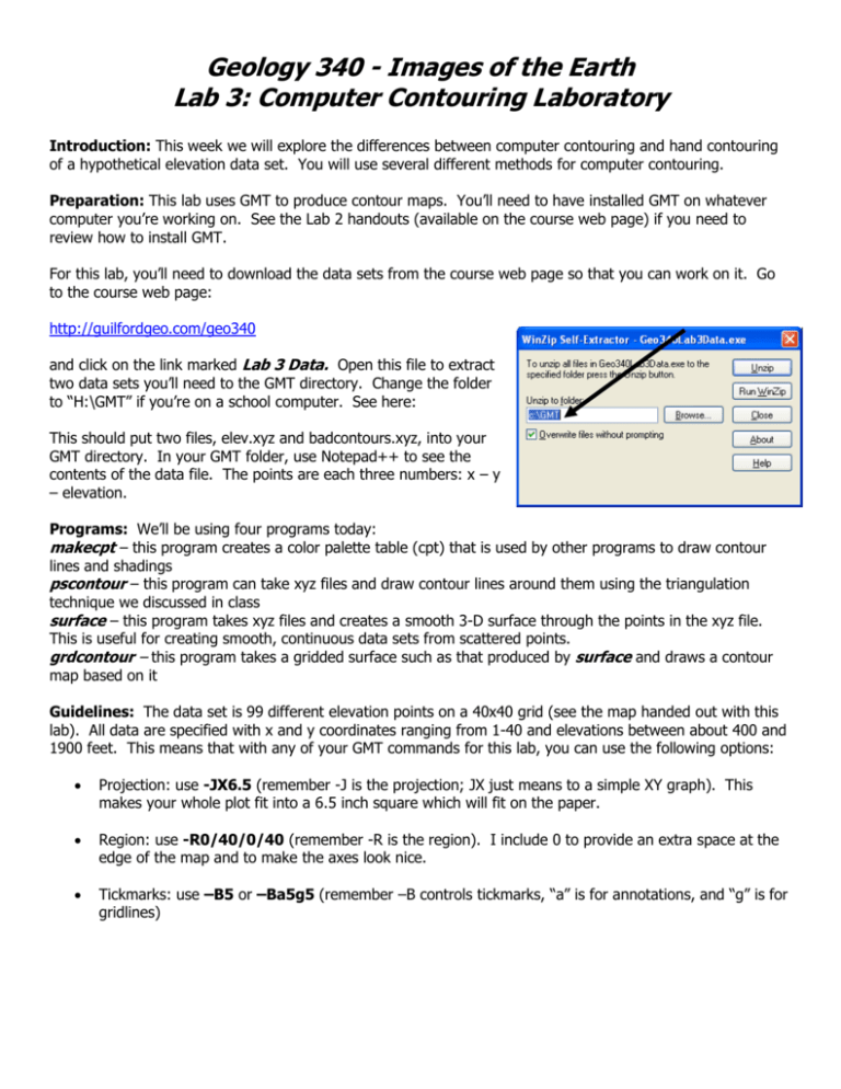
Geology 340 - Images of the Earth
Lab 3: Computer Contouring Laboratory
Introduction: This week we will explore the differences between computer contouring and hand contouring
of a hypothetical elevation data set. You will use several different methods for computer contouring.
Preparation: This lab uses GMT to produce contour maps. You’ll need to have installed GMT on whatever
computer you’re working on. See the Lab 2 handouts (available on the course web page) if you need to
review how to install GMT.
For this lab, you’ll need to download the data sets from the course web page so that you can work on it. Go
to the course web page:
http://guilfordgeo.com/geo340
and click on the link marked Lab 3 Data. Open this file to extract
two data sets you’ll need to the GMT directory. Change the folder
to “H:\GMT” if you’re on a school computer. See here:
This should put two files, elev.xyz and badcontours.xyz, into your
GMT directory. In your GMT folder, use Notepad++ to see the
contents of the data file. The points are each three numbers: x – y
– elevation.
Programs: We’ll be using four programs today:
makecpt – this program creates a color palette table (cpt) that is used by other programs to draw contour
lines and shadings
pscontour – this program can take xyz files and draw contour lines around them using the triangulation
technique we discussed in class
surface – this program takes xyz files and creates a smooth 3-D surface through the points in the xyz file.
This is useful for creating smooth, continuous data sets from scattered points.
grdcontour – this program takes a gridded surface such as that produced by surface and draws a contour
map based on it
Guidelines: The data set is 99 different elevation points on a 40x40 grid (see the map handed out with this
lab). All data are specified with x and y coordinates ranging from 1-40 and elevations between about 400 and
1900 feet. This means that with any of your GMT commands for this lab, you can use the following options:

Projection: use -JX6.5 (remember -J is the projection; JX just means to a simple XY graph). This
makes your whole plot fit into a 6.5 inch square which will fit on the paper.

Region: use -R0/40/0/40 (remember -R is the region). I include 0 to provide an extra space at the
edge of the map and to make the axes look nice.

Tickmarks: use –B5 or –Ba5g5 (remember –B controls tickmarks, “a” is for annotations, and “g” is for
gridlines)
Exercises:
1) Contour the data set provided by hand on the paper map. Use a 100-foot contour interval. Assume that
the numbered elevations apply at the center of the number.
2) Contour the data set by computer using the pscontour command. First, you'll need to use the makecpt
command to create a 100-foot contour cpt file. Cpt files are color/contour interval tables - see the
makecpt documentation for details. Your command might look something like this:
makecpt -Ccopper -T0/2000/100 > mycontours.cpt
Next, use the pscontour command to produce your contour map using triangulation. You'll need to
specify your data file (in this case elev.xyz) and then the -J, -R, and -B options (see last page) to get it to
work, and you'll need the -C option to specify your cpt file from the previous step. You also need to use –I
and –W to decide how to display the contours. Your command might looks something like this:
pscontour elev.xyz –JX6.5 –R0/40/0/40 –B5 –Cmycontours.cpt –I > map1.ps
Create one map with colored zones and one with contour lines (you'll need to switch the -I and -W options
to go from colors to lines).
3) QUESTION TO ANSWER: How does your hand-contoured map compare with this computer-contoured
map? Which do you think is more accurate? Where is each of these strongest? What errors does each
have?
4) Now use the surface and grdcontour commands to produce a second computer contour map from
gridded data. surface takes xyz data (your file elev.xyz) and creates a gridded elevation model using a
3-D spline. In the surface command, use a tension factor of zero (-T0) for now, and use an increment
both x and y of 1 (-I1), and you’ll need to specify an output grid file with the –G option (e.g. –Gelev.grd).
To make a map from the surface you created, use the grdcontour command, which makes a contour map
from the surface. In the grdcontour command, annotate the contours (-A100).
 QUESTION TO ANSWER: How does this contour map compare to the ones you produced in #2
above? Which do you think is more accurate?
 If you’re feeling adventuresome, you can create a colored image of the surface using the grdimage
command, which takes the same parameters as grdcontour except that it requires that the –C option
name a cpt file, as in –Cmycontours.cpt
5) Produce a second map using surface and grdcontour with a tension factor (-T) of 0.6. What differences
can you spot from the previous map (#4)?
6) Create another contour map using makecpt and pscontour, but this time use a contour interval of 20
feet. You should be able to use the same command as in problem #2, just with a different contour
interval specified in the makecpt command. How does the map look? Is this level of detail warranted
from the data you started with?
7) Look at the map labeled Scarp. Do a quick contour map by hand on the sheet provided.
8) The data for the Scarp map are in the file called badsurface.xyz. Do a line contour map using
pscontour.
9) Run this file through surface and grdcontour using a tension factor (-T) of zero. Notice anything weird?
What is going on here?
10) Repeat the mapping using a tension factor of 0.5 - how much does that mitigate the problem?