Supplemental Online Appendix
This appendix contains additional details about the statistical methods used in the main text.
Bivariate probit model
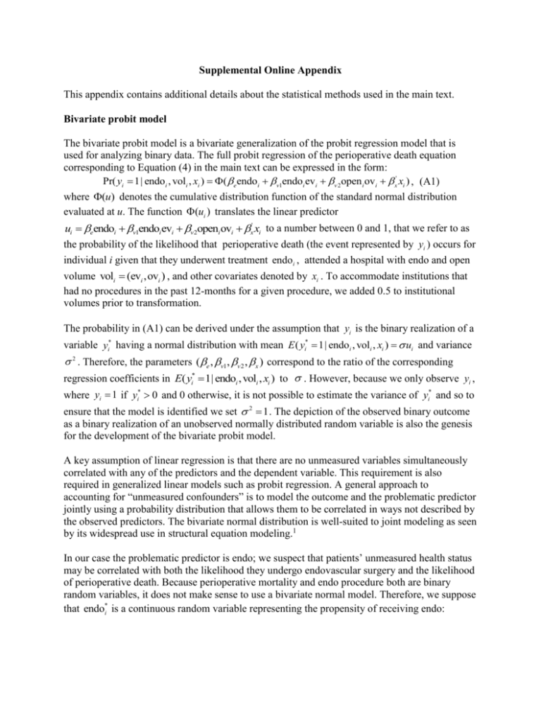
The bivariate probit model is a bivariate generalization of the probit regression model that is
used for analyzing binary data. The full probit regression of the perioperative death equation
corresponding to Equation (4) in the main text can be expressed in the form:
Pr( yi  1| endoi , voli , xi )  (  e endoi   v1endoi evi  v 2open i ovi   x' xi ) , (A1)
where (u) denotes the cumulative distribution function of the standard normal distribution
evaluated at u. The function  (ui ) translates the linear predictor
ui  eendoi  v1endoi evi  v 2openi ovi  x' xi to a number between 0 and 1, that we refer to as
the probability of the likelihood that perioperative death (the event represented by yi ) occurs for
individual i given that they underwent treatment endoi , attended a hospital with endo and open
volume voli  (evi ,ovi ) , and other covariates denoted by xi . To accommodate institutions that
had no procedures in the past 12-months for a given procedure, we added 0.5 to institutional
volumes prior to transformation.
The probability in (A1) can be derived under the assumption that yi is the binary realization of a
variable yi* having a normal distribution with mean E ( yi*  1| endoi , voli , xi )   ui and variance
 2 . Therefore, the parameters (e , v1, v 2 , x ) correspond to the ratio of the corresponding
regression coefficients in E( yi*  1| endoi , voli , xi ) to  . However, because we only observe yi ,
where yi  1 if yi*  0 and 0 otherwise, it is not possible to estimate the variance of yi* and so to
ensure that the model is identified we set  2  1 . The depiction of the observed binary outcome
as a binary realization of an unobserved normally distributed random variable is also the genesis
for the development of the bivariate probit model.
A key assumption of linear regression is that there are no unmeasured variables simultaneously
correlated with any of the predictors and the dependent variable. This requirement is also
required in generalized linear models such as probit regression. A general approach to
accounting for “unmeasured confounders” is to model the outcome and the problematic predictor
jointly using a probability distribution that allows them to be correlated in ways not described by
the observed predictors. The bivariate normal distribution is well-suited to joint modeling as seen
by its widespread use in structural equation modeling.1
In our case the problematic predictor is endo; we suspect that patients’ unmeasured health status
may be correlated with both the likelihood they undergo endovascular surgery and the likelihood
of perioperative death. Because perioperative mortality and endo procedure both are binary
random variables, it does not make sense to use a bivariate normal model. Therefore, we suppose
that endo*i is a continuous random variable representing the propensity of receiving endo:
endoi  1 if endo*i  0 and 0 otherwise. The bivariate probit model corresponding to the withinprocedure model (our selected model) is given by
'

 yi* 
 eendoi  v1endoi evi  v 2open i ovi   x xi   1  


N

,
2 
 , (A2)
*
'
v1pvi  v 2 tvi   x xi

 endoi 
   1 


where N2 denotes bivariate normal distribution, (pvi , tvi ) denotes the proportion of endo
procedures and total volume respectively, and  is the correlation representing the association
between yi* and endo*i induced by any unmeasured confounders. (For simplicity, the Box-Cox
transformation parameters are omitted from (A2).)
Parameter estimates are obtained for the model in (A2) by using the fact that the four bivariate
probabilities Pr( yi  a, endoi  b | endoi , voli , xi ) for (a, b)  {(0,0),(0,1),(1,0),(1,1)} depend on
the model parameters (e , v1 , v 2 ,  x , v1 , v 2 ,  x ,  ) . Thus, the frequency of occurrence of the
four bivariate binary observations can be related to the values of the predictors in order to find
the best-fitting values of the model parameters in both equations simultaneously. For more
extensive review of the bivariate probit model (and related models) we refer readers to
Heckman,2 Maddala,3 Mroz,4 and Bhattacharya, Goldman and McCaffrey.5
Box-Cox transformation
The Box-Cox transformation with parameter  of a variable v  0 is the function
(v  1) /  if   0
v( )  
.
(A3)
 log(v) if   0
There are several special cases including the linear, quadratic, and cubic (  1,2,3) ; the square
root and the cubed root (  1/ 2,1/ 3) ; the logarithm (  0) and the inverse square root, inverse
two-thirds power; and the inverse (  1/ 2, 2 / 3, 1) . An advantage of a parametric function
such as the Box-Cox transformation is that it lets the data decide which of these (and other)
transformations is most appropriate given the observed data and the assumed model, as opposed
to using an ad hoc method for choosing the transformation.
The parameter  can be estimated by using mathematical optimization routines to search for the
value that is most supported by the data under the assumed model. However, complications arise
because  is nonlinear (seen from the fact that the derivative of v( ) with respect to  is a
function of  ) and so numerical methods are needed for estimation. In practice,  is often preestimated and the ensuing analysis ignores the fact that  had to be estimated. A preferable
approach is to account for the uncertainty in  by embedding estimation of  with estimation of
the rest of the model. To our knowledge, Proc Qlim in SAS version 9.1 (and later versions) is the
only available procedure for fitting a bivariate probit model with embedded Box-Cox
transformations of the predictors.
In our analyses we used Box-Cox transformations of institutional volume for four primary
reasons: 1) it provides an easily interpretable overall measure of the shape of the volumeoutcome relationship; 2) we believed that the volume outcome relationship is monotone and
wanted to constrain the model as such; 3) we have multiple volume predictors (up to four in the
outcome equation) and are concerned that the models would get past the point of easy
interpretability if we used a separate spline model for each; 4) the availability of a SAS
procedure (Proc Qlim in SAS version 9.1) for fitting bivariate probit models with Box-Cox
transformed predictors simplified implementation of the model. An alternative to using a BoxCox transformation would be to use a semi-parametric representation of volume in the model.
The R statistical package SemiParBIVProbit (available at http://cran.rproject.org/web/packages/SemiParBIVProbit/) fits bivariate probit models involving semiparametric predictors.
Bayesian information criterion
A consequence of the fact that the bivariate probit model is nonlinear in the parameters is that R2
is no longer an appropriate metric to evaluate model fit. The Bayesian information criterion
(BIC) not only generalizes R2 to more general models but also guards against over-fitting. The
general mathematical definition of the BIC is:
BIC  q log(n)  2i1 log(p( yi ,endoi | evi ,ovi ,pvi , tvi , xi )) ,
n
(A4)
where q is the number of unknown parameters in the model and p ( yi , endoi | evi , ovi , pvi , tvi , xi )
is the probability density function (PDF) evaluated on the ith observation.
The BIC is verbalized as the number of model parameters times the log of the sample size minus
two times the log-likelihood function of the observed data. In the case of a linear regression
model, maximizing the log-likelihood function in (A4) is equivalent to maximizing R2. Because
better fitting models have greater likelihood function values, smaller values of BIC indicate
better model fit.
Adding more predictors to a model (increasing q) will always improve model fit and thus the
value of the log-likelihood function. However, in adherence to the principle of parsimony (e.g.,
Ockham’s razor), of two equally well-fitting models, one should favor the more parsimonious
model (usually the model with fewer parameters that the data is required to estimate). The BIC
endorses this belief through the q log(n) term which increases with q and, therefore, acts as a
penalty for the complexity of the model; the greater the value of q the greater the penalty. The
BIC is available as a model fit criterion in most major statistical packages.
Minimizing the BIC is one strategy for determining which model fits the data the best in
practice. Although we did not treat minimizing BIC as the ultimate criterion, it turned out that
our selected model (the within-volume model) had the lowest BIC even though the within- and
cross-volume model had more predictors.
References
1. Lee S-Y. Structural Equation Modeling: A Bayesian Approach [Chapter 2]. New York:
Wiley; 2007
2. Heckman JJ. Dummy Endogenous Variables in a Simultaneous Equation System.
Econometrica 1978;46:931-960
3. Maddala GS. Limited Dependent and Qualitative Variables in Econometrics.
Cambridge, UK: Cambridge University Press; 1983
4. Mroz T. Discrete factor approximations in simultaneously equation models: estimating
the impact of a dummy endogeneous variable on a continuous outcome. Journal of Econometrics
1999;93:54-62
5. Bhattacharya J, Goldman D, McCaffrey D. Estimating probit models with selfselected treatments. Statistics in Medicine 2006;25:389-413
Supplementary Tables
In the models presented in Table 2 (main text), different specifications are used for the functions
f (endoi , voli ; e , v ) and g (voli ;  v ) in Equation (1) and Equation (2) (main text). The specifications vary in
which predictors are included and also in the involvement of Box-Cox transformations. Let ee , oo , eo , oe ,
and tot demote the Box-Cox transformation parameters for endo volume on endo patients, open volume on
open patients, endo volume on open patients, open volume on endo patients, and total (endo and open) volume
on all patients respectively. The four models presented in Table 2 (main text) an in Tables A2 – A5 below are
distinguished as indicated in Table A1.
Table A1: Key regression models fit during model building process
Model
Non-clinical
Perioperative death: f (endoi , voli ; e , v )
Endo: g (voli ;  v )
Clinical adjusters
Excluded
0
0
+ Non-clinical
Included
0
0
+ Within volume
Included
 v1evi( ee ) endoi  v 2ovi( oo ) open i
 v1pei  v 2 tvi( tot )
+ Cross volume
Included
 (v1evi(ee )  v3ovi(eo ) )endoi  (v 4evi(oe )  v 2ovi(oo ) )openi
 v1pei  v 2 tvi( tot )
Note: The non-clinical adjusters (including date of procedure) are included in both or excluded from both the
endo and mortality equations.
Tables A2 – A5 contain the estimated model parameters for all the terms in Models 1 – 4
presented in Table 2 of the main text.
Table A2: Parameter estimates of regression coefficients for model with only clinical adjusters
Optimal Volume (Model 1)
Only clinical adjusters
Periop equation
Term
Endo Equation
Estimate 95% Conf Int Estimate 95% Conf Int
Key predictors
Endovascular repair
-0.710 (-1.275, -0.144)
Patient characteristics
Intercept
Age 70-74 (baseline 67-69)
Age 75-79 (baseline 67-69)
Age 80 & over (baseline 67-69)
Male
Black
End stage renal disease (ESRD)
-1.840 (-2.006, -1.674)
0.141 (0.065, 0.217)
0.296 (0.219, 0.374)
-0.834 (-0.873, -0.795)
0.064 (0.031, 0.096)
0.151 (0.118, 0.183)
0.555 (0.449, 0.661)
0.404
(0.370, 0.437)
-0.108 (-0.207, -0.009)
0.048 (-0.063, 0.159)
0.781 (0.623, 0.938)
0.385
(0.360, 0.410)
0.037 (-0.025, 0.100)
0.335 (0.218, 0.452)
0.317 (0.235, 0.400)
-0.040 (-0.093, 0.012)
Coronary bypass surgery (CABG)
-0.244 (-0.360, -0.128)
PTCA
-0.176 (-0.286, -0.067)
0.014 (-0.040, 0.067)
0.273 (0.210, 0.336)
-0.295 (-0.341, -0.248)
0.095 (0.047, 0.143)
0.050 (0.021, 0.078)
Chronic renal insufficiency
CAD without procedure
Chronic heart failure (CHF)
COPD
Vascular disease
Prior AAA diagnosis
0.125 (0.082, 0.168)
0.137 (0.087, 0.186)
-0.071 (-0.181, 0.040)
The estimated selection effect is 0.104 (0.252, 0.459) .
0.174
(0.142, 0.205)
0.030
(0.007, 0.052)
-0.099 (-0.122, -0.076)
0.449 (0.426, 0.471)
Table A3: Parameter estimates of regression coefficients for model adjusting for clinical and
non-clinical adjusters, reason and source of admission
Periop equation
Term
Endo Equation
Estimate 95% Conf Int Estimate 95% Conf Int
Key predictors
Endovascular repair
-0.707 (-1.186, -0.229)
Non-Clinical Adjusters
Procedure date
0.015
(0.014, 0.016)
Procedure date (Endo pats)
-0.004 (-0.008, -0.001)
Procedure date (Open pats)
0.001 (-0.003, 0.004)
Urgent Admission
0.293 (0.167, 0.419)
-0.504 (-0.558, -0.451)
Transfer
0.760 (0.572, 0.949)
-0.059 (-0.215, 0.096)
-1.877 (-2.005, -1.750)
0.138 (0.063, 0.214)
0.298 (0.222, 0.373)
-1.179 (-1.223, -1.136)
0.078 (0.045, 0.111)
0.162 (0.129, 0.195)
Patient characteristics
Intercept
Age 70-74 (baseline 67-69)
Age 75-79 (baseline 67-69)
Age 80 & over (baseline 67-69)
Male
Black
End stage renal disease (ESRD)
0.557 (0.463, 0.652)
0.417
-0.081 (-0.170, 0.009)
0.030 (-0.082, 0.142)
0.780 (0.627, 0.932)
0.387
(0.383, 0.451)
(0.361, 0.412)
0.056 (-0.007, 0.119)
0.357 (0.238, 0.476)
0.312 (0.227, 0.397)
-0.073 (-0.126, -0.020)
Coronary bypass surgery (CABG)
-0.253 (-0.362, -0.145)
PTCA
-0.159 (-0.265, -0.052)
0.017 (-0.038, 0.072)
0.271 (0.211, 0.331)
-0.273 (-0.320, -0.226)
0.001 (-0.047, 0.050)
0.081 (0.053, 0.109)
Chronic renal insufficiency
CAD without procedure
Chronic heart failure (CHF)
COPD
Vascular disease
Prior AAA diagnosis
0.123 (0.080, 0.166)
0.135 (0.085, 0.184)
-0.002 (-0.095, 0.091)
The estimated selection effect is 0.193 (0.112, 0.497) .
0.189
(0.157, 0.221)
0.028
(0.005, 0.051)
-0.105 (-0.128, -0.082)
0.417 (0.394, 0.441)
Table A4: Parameter estimates of regression coefficients for model adjusting for clinical and
non-clinical adjusters, reason and source of admission, and volume for procedure (the withinvolume model, our preferred model)
Periop equation
Term
Endo Equation
Estimate 95% Conf Int Estimate 95% Conf Int
Key predictors
Endovascular repair
-0.242 (-0.465, -0.020)
Proportion Endo
#
BC(Total volume)
λ(Total Volume)
3.004
(2.942, 3.065)
1.408
(1.309, 1.507)
-0.671 (-0.764, -0.579
#
BC(Endo volume, Endo pats)
-0.130 (-0.178, -0.082)
#
BC(Open volume, Open pats)
-0.066 (-0.082, -0.049)
λ(Endo Volume, Endo pats)
λ(Open volume, Open pats)
-0.153 (-0.516, 0.209)
0.136 (-0.229, 0.501)
Non-Clinical Adjusters
Procedure date
0.002
Procedure date (Endo pats)
-0.006 (-0.009, -0.003)
Procedure date (Open pats)
-0.003 (-0.005, -0.001)
(0.001, 0.003)
Urgent Admission
0.364 (0.290, 0.438)
-0.443 (-0.502, -0.384)
Transfer
0.815 (0.629, 1.001)
-0.162 (-0.326, 0.003)
-1.646 (-1.805, -1.488)
-3.718 (-4.008, -3.428)
Patient characteristics
Intercept
Age 70-74 (baseline 67-69)
0.127 (0.052, 0.203)
0.076
(0.040, 0.111)
Age 75-79 (baseline 67-69)
0.273 (0.199, 0.346)
0.162
(0.126, 0.198)
Age 80 & over (baseline 67-69)
0.487 (0.413, 0.562)
0.414
(0.377, 0.451)
Male
-0.147 (-0.193, -0.100)
0.399
(0.371, 0.426)
Black
0.005 (-0.108, 0.117)
0.005 (-0.063, 0.074)
End stage renal disease (ESRD)
0.728 (0.578, 0.877)
0.290
Chronic renal insufficiency
0.331 (0.249, 0.413)
-0.105 (-0.163, -0.048)
Coronary bypass surgery (CABG)
-0.201 (-0.302, -0.101)
-0.286 (-0.337, -0.236)
PTCA
-0.154 (-0.262, -0.047)
-0.030 (-0.083, 0.022)
(0.162, 0.418)
CAD without procedure
0.009 (-0.044, 0.062)
0.065
(0.034, 0.095)
Chronic heart failure (CHF)
0.245 (0.190, 0.300)
0.180
(0.146, 0.215)
COPD
0.115 (0.072, 0.158)
0.037
(0.012, 0.062)
Vascular disease
0.156 (0.113, 0.199)
Prior AAA diagnosis
-0.077 (-0.124, -0.030)
-0.137 (-0.162, -0.112)
0.410
(0.384, 0.435)
The estimated selection effect is 0.123 (0.189, 0.057) . The confidence intervals for these
effects were computed conditional on the corresponding Box-Cox transformation parameters.
Because the different transformation parameters make it difficult to assess which of endo and
open volume has greater impact on perioperative mortality, we refit the model using log volume
in the perioperative mortality equation (i.e., forcing the transformation parameters to equal 0).
The resulting within-volume coefficients were .092 (.126, .057) and .098 (.122, .074)
for endo and open, respectively, suggesting that the effects are on average similar in magnitude
across procedures.
#
Table A5: Parameter estimates of regression coefficients for model adjusting for clinical and
non-clinical adjusters, reason and source of admission, and volume for procedure and for the
other procedure (the within- and cross-volume model)
Periop equation
Term
Endo Equation
Estimate 95% Conf Int Estimate 95% Conf Int
Key predictors
Endovascular repair
-0.315 (-1.076, 0.446)
Proportion Endo
#
BC(Total volume)
λ(Total Volume)
3.004
(2.943, 3.064)
1.409
(1.310, 1.508)
-0.671 (-0.764, -0.579)
#
BC(Endo volume, Endo pats)
-0.112 (-0.204, -0.020)
#
BC(Open volume, Open pats)
-0.072 (-0.131, -0.012)
#
0.003 (-0.057, 0.064)
#
BC(Open volume, Endo pats)
-0.003 (-0.018, 0.012)
&
-0.153 (-0.516, 0.209)
&
λ(Open volume, Open pats)
0.136 (-0.229, 0.501)
λ(Endo volume, Open pats)
λ(Open volume, Endo pats)
0.647 (-3.473, 4.768)
BC(Endo volume, Open pats)
λ(Endo Volume, Endo pats)
0.436 (-1.678, 2.550)
Non-Clinical Adjusters
Procedure date
0.002
Procedure date (Endo pats)
-0.006 (-0.009, -0.003)
Procedure date (Open pats)
-0.003 (-0.005, -0.001)
(0.001, 0.003)
Urgent Admission
0.358 (0.273, 0.443)
-0.442 (-0.501, -0.384)
Transfer
0.805 (0.615, 0.994)
-0.162 (-0.326, 0.003)
-1.631 (-1.806, -1.457)
0.129 (0.053, 0.205)
0.276 (0.199, 0.353)
-3.719 (-3.860, -3.579)
0.075 (0.039, 0.111)
0.162 (0.126, 0.197)
Patient characteristics
Intercept
Age 70-74 (baseline 67-69)
Age 75-79 (baseline 67-69)
Age 80 & over (baseline 67-69)
Male
Black
End stage renal disease (ESRD)
0.496 (0.401, 0.590)
0.414
(0.377, 0.451)
-0.141 (-0.207, -0.075)
0.004 (-0.109, 0.116)
0.739 (0.581, 0.896)
0.399
(0.371, 0.427)
0.008 (-0.061, 0.076)
0.289 (0.161, 0.416)
0.333 (0.251, 0.415)
-0.106 (-0.164, -0.049)
Coronary bypass surgery (CABG)
-0.208 (-0.316, -0.099)
-0.286 (-0.337, -0.236)
PTCA
-0.157 (-0.265, -0.049)
0.010 (-0.044, 0.064)
0.248 (0.187, 0.309)
-0.030 (-0.082, 0.022)
0.065 (0.034, 0.095)
0.180 (0.146, 0.215)
Chronic renal insufficiency
CAD without procedure
Chronic heart failure (CHF)
COPD
Vascular disease
Prior AAA diagnosis
0.116 (0.072, 0.160)
0.153 (0.107, 0.200)
-0.071 (-0.138, -0.004)
0.037
(0.012, 0.062)
-0.137 (-0.162, -0.112)
0.410 (0.384, 0.435)
The estimated selection effect is 0.086 (0.354, 0.181) . #The confidence intervals for these
effects were computed conditional on the corresponding Box-Cox transformation parameters.
&
To help with identification of the model, the Box-Cox transformation parameters of the within
procedure volume variables are fixed at the estimates obtained under the within-procedure
model.