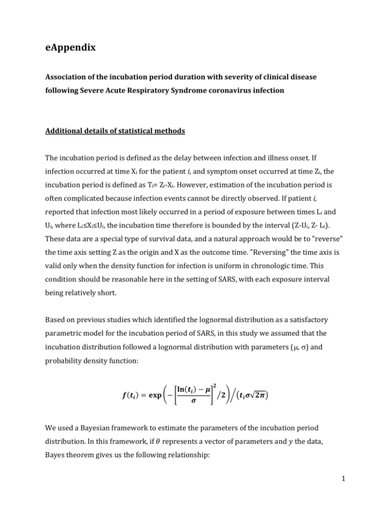
eAppendix
Association of the incubation period duration with severity of clinical disease
following Severe Acute Respiratory Syndrome coronavirus infection
Additional details of statistical methods
The incubation period is defined as the delay between infection and illness onset. If
infection occurred at time Xi for the patient i, and symptom onset occurred at time Zi, the
incubation period is defined as Ti= Zi-Xi. However, estimation of the incubation period is
often complicated because infection events cannot be directly observed. If patient i,
reported that infection most likely occurred in a period of exposure between times Li and
Ui, where Li≤Xi≤Ui, the incubation time therefore is bounded by the interval (Z-Ui, Z- Li).
These data are a special type of survival data, and a natural approach would be to "reverse"
the time axis setting Z as the origin and X as the outcome time. "Reversing" the time axis is
valid only when the density function for infection is uniform in chronologic time. This
condition should be reasonable here in the setting of SARS, with each exposure interval
being relatively short.
Based on previous studies which identified the lognormal distribution as a satisfactory
parametric model for the incubation period of SARS, in this study we assumed that the
incubation distribution followed a lognormal distribution with parameters (, ) and
probability density function:
𝟐
𝐥𝐧(𝒕𝒊 ) − 𝝁
𝒇(𝒕𝒊 ) = 𝐞𝐱𝐩 (− [
] ⁄𝟐)⁄(𝒕𝒊 𝝈√𝟐𝝅)
𝝈
We used a Bayesian framework to estimate the parameters of the incubation period
distribution. In this framework, if 𝜃 represents a vector of parameters and 𝑦 the data,
Bayes theorem gives us the following relationship:
1
(1)
𝒑(𝒚|𝜽)𝒑(𝜽)
𝒑(𝜽|𝒚) =
𝒑(𝒚)
where 𝑝(𝜃) is the prior probability of the parameters 𝜃 , 𝑝(𝑦|𝜃) is the likelihood function
and 𝑝(𝜃|𝑦) is the posterior probability of 𝜃 given the data 𝑦.
The MCMC process was initiated by giving random values to the parameters 𝜃 and by
choosing non-informative prior (flat prior) for 𝜃. A Metropolis Hastings algorithm was used
to update the parameter values in each iteration. In each iteration, all the 𝑘 parameters are
𝑗−1
randomly generated using the normal distribution with the mean 𝜃𝑘
𝑗−1
the kth parameter) and standard error 𝜎𝑘 , 𝑁(𝜃𝑘
(previous value of
, 𝜎𝑘 ) for each parameter. The updated
likelihood is compared with the previous one using the following accept-reject method:
𝒒=
𝒑(𝒚|𝜃 𝑗 )𝒑(𝜃 𝑗 )
𝒑(𝒚|𝜃 𝑗−1 )𝒑(𝜃 𝑗−1 )
If 𝑞 ≥ 1, the proposed new values of parameters 𝜃 𝑗 are accepted
If 𝑞 < 1, then 𝜃 𝑗 are accepted with probability 𝑞.
A burn-in period with 5,000 iterations was used to reduce the bias of the choice of the
initial parameter values and to generate values only in the stationary distribution. The
above algorithm was repeated 10,000 times after the burn-in period, with an acceptance
rate included in [0.45,0.55] for each parameter (adjusting on 𝜎𝑘 ).
For interval-censored data the following 𝑝(𝑦|𝜃) was used:
𝒏
𝒑(𝒚|𝜽) = ∏ 𝑺(𝒖𝒊 |𝜽) − 𝑺(𝒍𝒊 |𝜽)
𝒊=𝟏
where [𝑢𝑖 , 𝑙𝑖 ] are the interval censored data of the patient i and S(.) is the survival
lognormal distribution function.
2
Parameters of the fitted lognormal distribution
In patients with exposure intervals data, the parameters of the lognormal distribution were
estimated with the MCMC approach in the fatal and non-fatal cases, respectively. The
estimates are for fatal cases: = 0.97 (95% CrI: 0.44, 1.38) and = 0.88 (95% CrI: 0.58, 1.34)
and for non-fatal cases: = 1.24 (95% CrI: 1.09, 1.37) and = 0.88 (95% CrI: 0.58, 1.34).
Among patients of the Amoy garden cohort, the parameters of the lognormal distribution
were estimated with the same approach approach. The estimates are for fatal cases: = 1.37
(95% CrI: 1.19, 1.54) and = 0.54 (95% CrI: 0.43, 0.68) and for non-fatal cases: = 1.59
(95% CrI: 1.53, 1.65) and = 0.51 (95% CrI: 0.46, 0.55).
Logistic regression model
The logistic regression model used in this study is based on the following equation:
𝒑𝒊
𝒍𝒏 (
) = 𝜷𝟎 + 𝜷𝟏 𝑿𝟏 (𝒊𝒏𝒄𝒖𝒃𝒂𝒕𝒊𝒐𝒏 𝒑𝒆𝒓𝒊𝒐𝒅) + 𝜷𝟐 𝑿𝟐 (𝒂𝒈𝒆) + 𝜷𝟑 𝑿𝟑 (𝒔𝒆𝒙)
𝟏 − 𝒑𝒊
+ 𝜷𝟒 𝑿𝟒 (𝒐𝒄𝒄𝒖𝒑𝒂𝒕𝒊𝒐𝒏)
where pi is the probability of death, i’s are the regression coefficients, estimated with
MCMC (using flat priors N(0,100000)) and Xi ’s the explanatory variables labeled directly in
the equation above.
For the patients with exposure data, we performed this analysis three different ways: (1)
with Ti as the imputed midpoint of exposure intervals; (2) with Ti as the mean of the 10,000
posterior samples i.e. simulated incubation times for each patient; (3) with Ti resampled
from the 10,000 posterior samples in each MCMC iteration. Results of these different
analyses are presented in eAppendix Table 1. Significant association between incubation
period and risk of death was observed using the mean approach (2) and the imputation
3
approach (3) whereas no significant association was observed with the midpoint
imputation method (1). The results of method (3) are presented in the main text, as this is
the most appropriate approach.
Sensitivity analyses
Sensitivity analyses were conducted in both subsets of patients. For the patients with
available exposure data, an interval of 0 to 20 days was selected for the main analysis due
to the data reported by some patients with very wide exposure intervals that are not
informative. As a sensitivity analysis, a subgroup of patients was extracted with an inclusion
criteria based on the exposure intervals of no more than 10 days (N=185). We also fitted
the logistic regression model for this subset of patients using the mean incubation time and
found very similar associations of the incubation period with risk of death (OR=0.77; 95%
CI: 0.53 - 1.04).
For the Amoy Gardens cluster of cases (eAppendix Figure 1), which were thought to have
been caused by a super-spreading event, we examined potential dates of common infection
for all members of the cluster and estimated that the most likely infection date was 21st
March 2003. A period of 14 days i.e. cases with onset dates between 22 March 2003 and 4
April 2003 (shown in eAppendix Figure 1) was selected for the main analysis in order to
exclude the small number of cases infected prior to the super-spreading event, and cases
that had symptom onset late in the outbreak and may have been secondary or tertiary
infections. We also conducted a sensitivity analysis using first a larger subset of patients,
with onset dates between 22 March 2003 and 10 April 2003 (N=320) and secondly using a
smaller subset with onset dates between 22 March 2003 and 31 April 2003 (N=286).
Results from the logistic regression model show similar associations of the incubation
period with risk of death (OR=0.92; 95% CI: 0.82-1.02 and OR=0.77; 95% CI: 0.62-0.94,
respectively).
4
To evaluate the potential cofounding effect of age, we conducted a stratified analysis using
two categories of age with the threshold of 50 years (eAppendix Table 2). A significant
association between incubation period and risk of death was only observed among Amoy
garden cohort patients. No significant association was observed for patients with exposure
data, probably due to the reduced sample size in the sub-analysis.
Moreover, to examine the sensitivity of our results to the assumption of a linear association
between incubation time and the log-odds of death, we conducted a similar analysis with a
logistic regression model described previously with the incubation period as a categorical
variable, using tertiles (eAppendix Table 3). We observed a significant association
between shorter incubation period and an increased risk of death only in the Amoy Garden
cohort. However, no significant association was observed in the cases of the exposure data
patients although the direction of point estimates was consistent with the analysis
presented in the main text.
5
eAppendix Table 1. Association between estimated incubation period (T) and risk of
death for each case of Severe Acute Respiratory Syndrome
Incubation period (Ti), per day
Risk of Death1
OR (95% CI)
Cases with reported exposure dates (n=234)
Midpoint imputation
0.89 (0.76 - 1.03)
Mean incubation time, T𝑖
0.84 (0.68 - 1.00)
Simulated incubation times2
0.86 (0.71 - 1.00)
Cases in the Amoy Gardens cluster (n=308)
Incubation period3
1
0.79 (0.67 - 0.94)
The odds ratios (exp()) were estimated using Markov Chain Monte Carlo (10,000 runs) to estimate the coefficients () of
the multivariable logistic regression model, with death status as the binary outcome variable and the incubation period, sex,
age and occupation as predictors.
2
10,000 samples from the posterior distributions of the two parameters (μ, σ) and the incubation periods T for each patient
were drawn using MCMC in the same algorithm in order to retain uncertainty in the incubation period in the analysis of
severity.
3
Incubation period estimated based on illness onset dates, with an assumed infection date for all cases of 21 March 2003.
6
eAppendix Table 2. Age stratified analysis of association between risk of death and
estimated incubation period, sex and occupation.
Risk of Death1
Cases
OR (95% CI)
Cases with reported exposure dates
(n=234)
Incubation period1
Cases in the Amoy Gardens cluster
(n=308)
Incubation period2
1
0 - 49 years old
50 years old
9/1633
16/463
0.91 (0.70 - 1.11)
0.91 (0.73 - 1.09)
22/2363
16/343
0.91 (0.65 - 0.98)
0.70 (0.65 - 0.92)
The odds ratios (exp()) were estimated using Markov Chain Monte Carlo (10,000 runs) to estimate the coefficients () of
the multivariable logistic regression model, with death status as the binary outcome variable and the incubation period, sex
and occupation as predictors. 10,000 samples from the posterior distributions of the two parameters (μ, σ) and the incubation
periods T for each patient were drawn using MCMC in the same algorithm in order to retain uncertainty in the incubation
period in the analysis of severity.
2
Incubation period estimated based on illness onset dates, with an assumed infection date for all cases of 21 March 2003.
3 number
of fatal cases/number of non-fatal cases
7
eAppendix Table 3. Association between estimated incubation period (T) using
categorical variables (tertiles) and risk of death for each case of Severe Acute
Respiratory Syndrome
Factors
Incubation period below 1st tertile
(shortest)1 (reference group)
Incubation period between 1st and
2nd tertile1
Incubation period above 2nd tertile
(longest)1
1
Risk of death, OR (95%
Risk of death, OR
CrI) in cases with
(95% CrI) in cases of
reported exposure
the Amoy Gardens
dates (n=234)
cluster (n=308)2
1.00
1.00
0.68 (0.22 - 2.11)
0.18 (0.05 - 0.63)
0.57 (0.17 - 1.73)
0.07 (0.02 - 0.27)
The odds ratios (exp()) were estimated using Markov Chain Monte Carlo (10,000 runs) to estimate the coefficients () of
the multivariable logistic regression model, with death status as the binary outcome variable and the incubation period, age,
sex and occupation as predictors. The tertiles were (2.3, 5.0 days) and (2.8, 5.8 days) for the patients with exposure data and
the Amoy garden cohort, respectively
2
Incubation period estimated based on illness onset dates, with an assumed infection date for all cases of 21 March 2003.
8
eAppendix Figure 1. Distribution of illness onset dates for all cases determined
through epidemiologic investigations to form the Amoy Gardens cluster (n=331). The
putative super spreading event happened on the 21st March 2003. The two vertical lines
delimit the period of selection for the patients included in the main analysis. The dotted line
indicates a lognormal distribution for the incubation period estimated on the separate
subset of cases with exposure information as shown in Figure 1A in the main text (i.e.
incubation period with mean 4.7 days, standard deviation 4.6 days).
Selected for analysis
0.25
Proportion of cases (%)
0.20
0.15
0.10
0.05
0.00
13/03
17/03
21/03
25/03
29/03
02/04
06/04
10/04
14/04
Calendar date of symptom onset, 2003
9