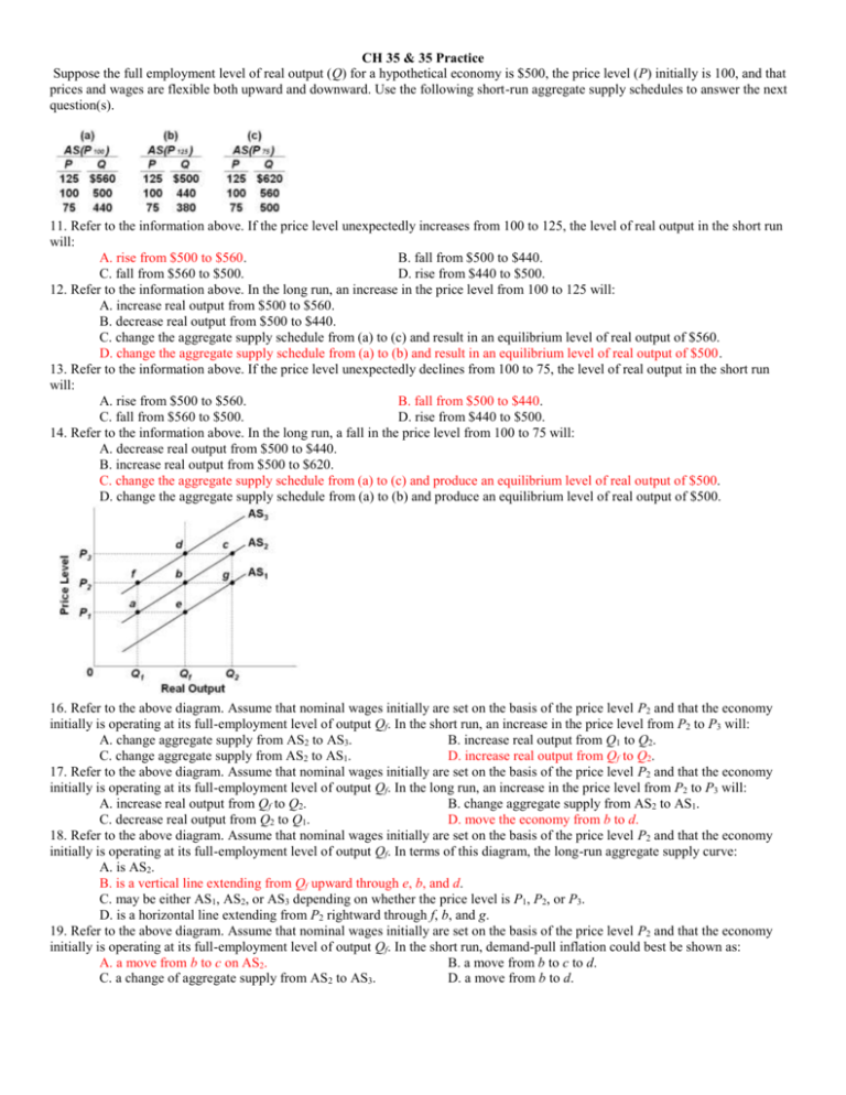
CH 35 & 35 Practice
Suppose the full employment level of real output (Q) for a hypothetical economy is $500, the price level (P) initially is 100, and that
prices and wages are flexible both upward and downward. Use the following short-run aggregate supply schedules to answer the next
question(s).
11. Refer to the information above. If the price level unexpectedly increases from 100 to 125, the level of real output in the short run
will:
A. rise from $500 to $560.
B. fall from $500 to $440.
C. fall from $560 to $500.
D. rise from $440 to $500.
12. Refer to the information above. In the long run, an increase in the price level from 100 to 125 will:
A. increase real output from $500 to $560.
B. decrease real output from $500 to $440.
C. change the aggregate supply schedule from (a) to (c) and result in an equilibrium level of real output of $560.
D. change the aggregate supply schedule from (a) to (b) and result in an equilibrium level of real output of $500.
13. Refer to the information above. If the price level unexpectedly declines from 100 to 75, the level of real output in the short run
will:
A. rise from $500 to $560.
B. fall from $500 to $440.
C. fall from $560 to $500.
D. rise from $440 to $500.
14. Refer to the information above. In the long run, a fall in the price level from 100 to 75 will:
A. decrease real output from $500 to $440.
B. increase real output from $500 to $620.
C. change the aggregate supply schedule from (a) to (c) and produce an equilibrium level of real output of $500.
D. change the aggregate supply schedule from (a) to (b) and produce an equilibrium level of real output of $500.
16. Refer to the above diagram. Assume that nominal wages initially are set on the basis of the price level P2 and that the economy
initially is operating at its full-employment level of output Qf. In the short run, an increase in the price level from P2 to P3 will:
A. change aggregate supply from AS2 to AS3.
B. increase real output from Q1 to Q2.
C. change aggregate supply from AS2 to AS1.
D. increase real output from Qf to Q2.
17. Refer to the above diagram. Assume that nominal wages initially are set on the basis of the price level P2 and that the economy
initially is operating at its full-employment level of output Qf. In the long run, an increase in the price level from P2 to P3 will:
A. increase real output from Qf to Q2.
B. change aggregate supply from AS2 to AS1.
C. decrease real output from Q2 to Q1.
D. move the economy from b to d.
18. Refer to the above diagram. Assume that nominal wages initially are set on the basis of the price level P2 and that the economy
initially is operating at its full-employment level of output Qf. In terms of this diagram, the long-run aggregate supply curve:
A. is AS2.
B. is a vertical line extending from Qf upward through e, b, and d.
C. may be either AS1, AS2, or AS3 depending on whether the price level is P1, P2, or P3.
D. is a horizontal line extending from P2 rightward through f, b, and g.
19. Refer to the above diagram. Assume that nominal wages initially are set on the basis of the price level P2 and that the economy
initially is operating at its full-employment level of output Qf. In the short run, demand-pull inflation could best be shown as:
A. a move from b to c on AS2.
B. a move from b to c to d.
C. a change of aggregate supply from AS2 to AS3.
D. a move from b to d.
23. Refer to the above diagram relating to short-run and long-run aggregate supply. The
A. short-run aggregate supply curve is A.
B. short-run aggregate supply curve is B.
C. long-run aggregate supply curve is B.
D. long-run aggregate supply curve is D.
24. Refer to the above diagram. If the price level rises above P1 because of an increase in aggregate demand, the:
A. economy will move up along curve B and output will temporarily increase.
B. long-run aggregate supply curve C will shift upward.
C. short-run aggregate supply curve B will automatically shift to the right.
D. economy's output first will decline, then increase, and finally return to Q1.
25. Refer to the above diagram. The long-run aggregate supply curve is:
A. A.
B. B.
C. C.
D. D.
26. Refer to the above diagram. The short-run aggregate supply is:
A. A.
B. B.
C. D.
D. not represented in the diagram.
27. Refer to the above diagram and assume the economy is operating at equilibrium point w. In the short run, an increase in the price
level from P2 to P3 would move the economy from point w to point:
A. v.
B. x.
C. u.
D. z.
28. Refer to the above diagram and assume the economy is operating at equilibrium point w. In the long run, an increase in the price
level from P2 to P3 would move the economy from point w to point:
A. v.
B. x.
C. u.
D. y.
29. Refer to the above diagram and assume the economy is operating at equilibrium point w. In the short run, a decrease in the price
level from P2 to P1 would move the economy from point w to point:
A. v.
B. x.
C. t.
D. y.
30. Refer to the above diagram and assume the economy is operating at equilibrium point w. If wages and other resource prices are
flexible downward, in the long run a decrease in the price level from P2 to P1 would move the economy from point w to point:
A. v.
B. x.
C. t.
D. y.
31. Refer to the above diagram. If drawn, the long-run aggregate supply curve would include points:
A. v, w, and u.
B. y, w, and u.
C. t, w, and z.
D. y, w, and x.
35. Refer to the above diagram. The initial aggregate demand curve is AD 1 and the initial aggregate supply curve is AS 1. Demand-pull
inflation in the short run is best shown as:
A. a shift of the aggregate demand curve from AD1 to AD2. B. a move from d to b to a.
C. a move directly from d to a.
D. a shift of the aggregate supply curve from AS1 to AS2.
36. Refer to the above diagram. The initial aggregate demand curve is AD 1 and the initial aggregate supply curve is AS 1. In the long
run, demand-pull inflation is best shown as:
A. a shift of aggregate demand from AD1 to AD2 followed by a shift of aggregate supply from AS1 to AS2.
B. a move from d to b to a.
C. a shift of aggregate supply from AS1 to AS2 followed by a shift of aggregate demand from AD1 to AD2.
D. a move from a to d.
37. Refer to the above diagram. The initial aggregate demand curve is AD 1 and the initial aggregate supply curve is AS 1. In the long
run, the aggregate supply curve is vertical in the diagram because:
A. nominal wages and other input prices are assumed to be fixed.
B. real output level Qf is the potential level of output.
C. price level increases produce perfectly offsetting changes in nominal wages and other input prices.
D. higher than expected rates of actual inflation reduce real output only temporarily.
38. Refer to the above diagram. The initial aggregate demand curve is AD 1 and the initial aggregate supply curve is AS 1. Cost-push
inflation in the short run is best represented as a:
A. leftward shift of the aggregate supply curve from AS1 to AS2.
B. rightward shift of the aggregate demand curve from AD1 to AD2.
C. move from d to b to a.
D. move from d directly to a.
39. Refer to the above diagram. The initial aggregate demand curve is AD 1 and the initial aggregate supply curve is AS 1. Assuming no
change in aggregate demand, the long-run response to a recession caused by cost-push inflation is best depicted as a:
A. move from a to d along the long-run aggregate supply curve.
B. rightward shift of the aggregate supply curve from AS2 to AS1.
C. move from a to c to d.
D. leftward shift of the aggregate supply curve from AS1 to AS2.
44. Refer to the above diagram and assume that prices and wages are flexible both upward and downward in the economy. In the
extended AD-AS model:
A. demand-pull inflation would involve a rightward shift of curve A, followed by a leftward shift of curve C.
B. cost-push inflation would involve a rightward shift of curve A, followed by a leftward shift of curve C.
C. recession would involve a leftward shift of curve A, followed by a leftward shift of curve C.
D. recession would involve a rightward shift of curve D, followed by leftward shifts of curves A and C.
45. Refer to the above diagram and assume that prices and wages are flexible both upward and downward in the economy. In the
extended AD-AS model:
A. demand-pull inflation would involve a rightward shift of curve A, followed by a rightward shift of curve C.
B. cost-push inflation would involve first a leftward shift of curve C, then a rightward shift of curve C.
C. recession would involve a leftward shift of curve A followed by a leftward shift of curve C.
D. recession would involve a rightward shift of curve D, followed by leftward shifts of curves A and C.
46. Refer to the above diagram and assume that prices and wages are flexible both upward and downward in the economy. In the
extended AD-AS model:
A. demand-pull inflation would involve a rightward shift of curve A, followed by a rightward shift of curve C.
B. cost-push inflation would involve a rightward shift of curve A, followed by a leftward shift of curve C.
C. recession would involve a leftward shift of curve A, followed by a rightward shift of curve C.
D. recession would involve a rightward shift of curve D, followed by leftward shifts of curves A and C.
47. Refer to the above diagram and assume that prices and wages are flexible both upward and downward in the economy. In the
extended AD-AS model:
A. demand-pull inflation would involve a rightward shift of curve A, followed by a rightward shift of curve C.
B. cost-push inflation would involve a rightward shift of curve A, followed by a leftward shift of curve C.
C. recession would involve a leftward shift of curve A, followed by a leftward shift of curves C and D.
D. recession could be caused by either a leftward shift of curve A or a leftward shift of curve C.
48. Refer to the above diagram and assume that prices and wages are flexible both upward and downward in the economy. In the
extended AD-AS model:
A. demand-pull inflation would involve a shift of curve D to the right.
B. cost-push inflation would involve a shift of curve B downward.
C. recession would involve a leftward shift of curve A.
D. frictional unemployment would be zero in the long run.
50. Refer to the above graphs. Curve AB is a:
A. production possibilities curve and curve X is a long-run aggregate supply curve.
B. consumer demand curve and curve X is a long-run aggregate supply curve.
C. long-run aggregate supply curve and Y is potential real GDP curve.
D. long-run aggregate supply curve and X is a production possibilities curve.
51. Refer to the above graphs. Growth of production capacity is shown by:
A. the shift from AB to CD only.
B. the shift from X to Y only.
C. both the shift from AB to CD and the shift from X to Y.
D. both the shift from AB to CD and the shift from Y to X.
52. Refer to the above graphs. An increase in an economy's labor productivity would shift curve:
A. AB to CD and shift curve Y to X.
B. CD to AB and shift curve X to Y.
C. AB to CD and shift curve X to Y.
D. X to Y while leaving curve AB in place.
53. Refer to the above graphs. An increase in the economy's human capital would shift curve:
A. AB to CD and curve Y to X.
B. CD to AB and curve X to Y.
C. X to Y while leaving curve AB in place.
D. AB to CD and curve X to Y.
56. Refer to the above graphs, where the subscripts on the labels denote years 1 and 2. In year 1 the economy:
A. is in long-run equilibrium at output Q1.
B. is in short-run equilibrium at output Q1, but not in long-run equilibrium.
C. cannot be in long-run equilibrium because output changes in period 2.
D. is in a recession, based on output Q1 being below output Q2.
57. Refer to the above graphs, where the subscripts on the labels denote years 1 and 2. From the graphs we can clearly conclude that
from year 1 to year 2:
A. the economy recovered from a recession.
B. the economy experienced economic growth and mild inflation.
C. output grew and the unemployment rate fell.
D. the government engaged in expansionary fiscal and monetary policies.
58. Refer to the above graphs, where the subscripts on the labels denote years 1 and 2. From the graphs we can clearly conclude that
the economy:
A. is not at full employment in either year.
B. is at full employment in year 1, but not in year 2.
C. is at full employment in year 2, but not in year 1.
D. is at full employment in both years.
62. Refer to the above diagram for a specific economy. The curve on this graph is known as a:
A. Laffer Curve.
B. Phillips Curve.
C. labor demand curve.
D. production possibilities curve.
63. Refer to the above diagram for a specific economy. Which of the following best describes the relationship shown by this curve?
A. The demand for labor is large when the rate of inflation is small.
B. When the rate of unemployment is high, the rate of inflation is high.
C. The rate of inflation and the rate of unemployment are inversely related.
D. The rate of inflation and the rate of unemployment are directly related.
64. Refer to the above diagram for a specific economy. A reduction in structural unemployment or bottleneck problems in labor
markets will:
A. shift this curve to the right.
B. shift this curve to the left.
C. move this economy southeast along the curve.
D. move this economy northwest along the curve.
65. Refer to the above diagram for a specific economy. An increase in aggregate demand will:
A. shift this curve to the right.
B. shift this curve to the left.
C. move this economy southeast along the curve.
D. move this economy northwest along the curve.
66. Refer to the above diagram for a specific economy. Which of the following best describes a decision by policymakers that moves
this economy from point b to point a?
A. Policymakers have instituted an expansionary monetary policy and/or a budgetary deficit, thereby accepting more
unemployment to reduce the rate of inflation.
B. Policymakers have instituted a restrictive monetary policy and/or a budgetary surplus, thereby accepting a higher rate of
inflation to reduce unemployment.
C. Policymakers have instituted an expansionary monetary and/or a budgetary deficit, thereby accepting a higher rate of
inflation to reduce unemployment.
D. Policymakers have instituted a restrictive monetary policy and/or a budgetary surplus, thereby accepting more
unemployment to reduce the rate of inflation.
89. The above diagram is the basis for explaining:
A. the traditional Phillips Curve.
B. the long-run Phillips Curve.
C. how central planning can make full employment and price level stability compatible goals.
D. new policies for eliminating unemployment.
90. Refer to the above diagram. The natural rate of unemployment for this economy is:
A. 3 percent.
B. 5 percent.
C. 6 percent.
D. 4 percent.
91. Refer to the above diagram. Assume the economy is initially at point b1. With a time lag between price and nominal wage
adjustments, an increase in aggregate demand will temporarily move the economy from:
A. b2 to b1.
B. c1 to b2.
C. b1 to c1.
D. b1 to b2.
92. Refer to the above diagram and assume the economy is initially at point b1. Which of the following movements is consistent with
the traditional Phillips Curve?
A. the movement from b1 to b2
B. the movement from b1 to c1
C. the movement from c1 to b2
D. the movement from b2 to b1
93. Refer to the above diagram and assume the economy is initially at point b1. Point c1 represents:
A. a stable position because reality and expectations are consistent.
B. a stable position because full employment and a constant annual inflation rate are represented.
C. an unstable situation because government will undertake contractionary policies.
D. an unstable situation because nominal wage rates will increase.
94. Refer to the above diagram and assume the economy is initially at point b1. The long-run relationship between the unemployment
rate and the rate of inflation is represented by:
A. the line connecting b1 and c1.
B. the line through b1, b2, b3, and b4.
C. the line connecting c1 and b2.
D. any line parallel to the horizontal axis.
97. Refer to the above diagram. Assume that the natural rate of unemployment is 5 percent and that the economy is initially operating
at point a where the expected and actual rates of inflation are each 6 percent. If the actual rate of inflation unexpectedly falls from 6
percent to 4 percent, then the unemployment rate will:
A. temporarily fall from 5 percent to 4 percent.
B. permanently fall from 5 percent to 4 percent.
C. temporarily rise from 5 percent to 7 percent.
D. permanently rise from 5 percent to 7 percent.
98. Refer to the above diagram. Assume that the natural rate of unemployment is 5 percent and that the economy is initially operating
at point a where the expected and actual rates of inflation are each 6 percent. In the long run, the decline in the actual rate of inflation
from 6 percent to 4 percent will:
A. reduce the unemployment rate.
B. reduce corporate profits in real terms.
C. have no effect on the unemployment rate.
D. reduce real domestic output.
99. Refer to the above diagram. Assume that the natural rate of unemployment is 5 percent and that the economy is initially operating
at point c where the expected and actual rates of inflation are each 4 percent. If the actual rate of inflation unexpectedly rises from 4
percent to 6 percent, the economy will:
A. move from a to b and eventually to c.
B. move directly from c to b.
C. remain at a.
D. move from c to d and eventually to a.
100. In the above diagram:
A. any rate of inflation is consistent with the natural rate of unemployment in the long run.
B. inflation can occur but disinflation cannot occur.
C. unemployment rates exceeding the natural rate are permanent.
D. unemployment rates less than the natural rate are permanent.
101. Refer to the above diagram. Point b on short-run Phillips Curve PC1 represents a rate of:
A. inflation below the natural rate.
B. inflation above the natural rate.
C. unemployment above the natural rate.
D. unemployment below the natural rate.
102. Refer to the above diagram. Point b would be explained by:
A. an actual rate of inflation that exceeds the expected rate.
B. an actual rate of inflation that is less than the expected rate.
C. cost-push inflation.
D. an increase in long-run aggregate supply.
103. Refer to the above diagram. Point b would not be permanent because the:
A. economy would move from b to a on PC1.
B. short-run Phillips Curve would shift from PC1 to PC2 and unemployment would increase to the natural rate at c.
C. economy would immediately move from b to c to d.
D. economy would move from b directly to d.
104. Refer to the above diagram. The move of the economy from c to e on short-run Phillips Curve PC2 would be explained by an:
A. increase in aggregate demand in the economy.
B. increase in aggregate supply in the economy.
C. actual rate of inflation that is less than the expected rate.
D. actual rate of inflation that exceeds the expected rate.
107. The above curve is known as the:
A. Taylor rule.
B. Okun Curve.
C. Laffer Curve.
D. Phillips Curve.
108. Refer to the above diagram. Supply-side economists believe that tax rates are:
A. such that an increase in tax rates will increase tax revenues.
B. at some level below b.
C. at some level above b.
D. at d.
109. In the above curve, a decline in the tax rate from c to b would:
A. greatly increase tax revenue.
B. greatly decrease tax revenue.
C. leave tax revenue about the same as before.
D. shift the curve to the left.
110. Refer to the above diagram. If the tax rate is currently c and the government wants to maximize tax revenue, it should:
A. leave the tax rate at c.
B. increase the tax rate to d.
C. reduce the tax rate to b.
D. reduce the tax rate to a.
Chapter 36
8. The basic equation of monetarism is:
A. MV = PQ.
B. Sa + T + M = Ig + G + Xn.
C. V = M/PQ.
D. Ca + Ig + Xn + G = GDP.
Answer the next question(s) on the basis of the following information for a hypothetical economy. All values are in nominal terms.
M = $100, V = 2, Ca = $160, Xn = $10, G = $10
25. Refer to the above information. Nominal GDP is:
A. $100.
B. $200.
26. Refer to the above information. If the price level P is 4, Q is:
A. 50.
B. 100.
27. Refer to the above information. In equilibrium, Ig is:
A. $20.
B. $10.
C. $180.
D. $50.
C. 200.
D. 500.
C. $5.
D. $50.
47. Refer to the above diagram. A decline of aggregate supply from AS LR1 to ASLR2, followed by a decline of aggregate demand from
AD1 to AD2, would best describe the:
A. direct relationship between aggregate supply and aggregate demand.
B. real-business-cycle view of recession.
C. monetarist view of recession.
D. mainstream, Keynesian-based, view of recession.
48. Refer to the above diagram. The real-business cycle view of recession would best be described by:
A. a decrease of aggregate demand from AD1 to AD2, followed by a decrease in aggregate supply from AS LR1 to ASLR2.
B. an increase in aggregate demand from AD1 to AD2, which in turn caused a decrease in aggregate supply from AS LR1 to
ASLR2.
C. a decrease in aggregate supply from ASLR1 to ASLR2, followed by a decrease in aggregate demand from AD 1 to AD2.
D. a decrease in aggregate supply from ASLR1 to ASLR2, followed by an increase in aggregate demand from AD2 to AD1.
58. Refer to the above diagram. Rational expectations theory says that a fully anticipated shift in aggregate demand from AD 1 to AD2
will:
A. move the economy from a to b to c.
B. move the economy directly from a to c.
C. move the economy from a to new equilibrium at b.
D. shift the AS curve to the right.
59. Refer to the above diagram. Rational expectations theory says that a fully anticipated decrease in aggregate demand from AD 2 to
AD1 will:
A. move the economy from a to b to c.
B. shift the AS curve to the left.
C. move the economy from c to new equilibrium b.
D. move the economy directly from c to a.
60. Refer to the above diagram. Suppose that, as expected, aggregate demand declines from AD 2 to AD1. A direct move of the
economy from c to a would best reflect:
A. new classical economics.
B. mainstream economics.
C. the real-business-cycle theory.
D. a coordination failure.
67. Refer to the above figure and assume the economy initially is in equilibrium at point a. In the new classical theory, an
unanticipated increase in aggregate demand from AD2 to AD1 would move the economy:
A. directly from a to d.
B. from a to b to d.
C. from a to e to d.
D. directly from a to f.
68. Refer to the above figure and assume the economy initially is in equilibrium at point a. In the new classical theory, a fully
anticipated increase in aggregate demand from AD2 to AD1 would move the economy:
A. directly from a to d.
B. from a to b to d.
C. from a to e to d.
D. directly from a to f.
69. Refer to the above figure and assume the economy initially is in equilibrium at point a. In the new classical theory, an
unanticipated decrease in aggregate demand from AD 2 to AD3 would move the economy:
A. directly from a to h.
B. from a to g to h.
C. directly from a to d.
D. from a to c to h.
70. Refer to the above figure and assume the economy initially is in equilibrium at point a. In the new classical theory, a fully
anticipated decrease in aggregate demand from AD2 to AD3 would move the economy:
A. directly from a to h.
B. from a to g to h.
C. directly from a to d.
D. from a to c to h.
76. Refer to the above diagram and assume the economy initially is in equilibrium at point a. In the mainstream view, a decline in
aggregate demand from AD1 to AD2 would likely move the economy:
A. directly from a to d.
B. directly from a to b.
C. from a to c, then quickly from c to d.
D. from a to c, then eventually from c to b.
77. Refer to the above diagram and assume the economy initially is in equilibrium at point a. Suppose the aggregate demand declines
from AD1 to AD2 and the economy moves from a to c. In the mainstream view, the resulting decline in the price level need not shift
the short-run aggregate supply curve from AS1 to AS2 because:
A. supply creates its own demand.
B. nominal wages are (at least for a time) inflexible downward.
C. firms misperceive the price-level decline as being permanent.
D. deflation reduces the purchasing power of the dollar.
81. Refer to the above table. At the $8 wage, labor cost per-unit of output is:
A. $1.25.
B. $1.50.
C. $2.00.
82. Refer to the above table. The efficiency wage is:
A. $10.
B. $9.
C. $8
D. $6.
D. $1.67.