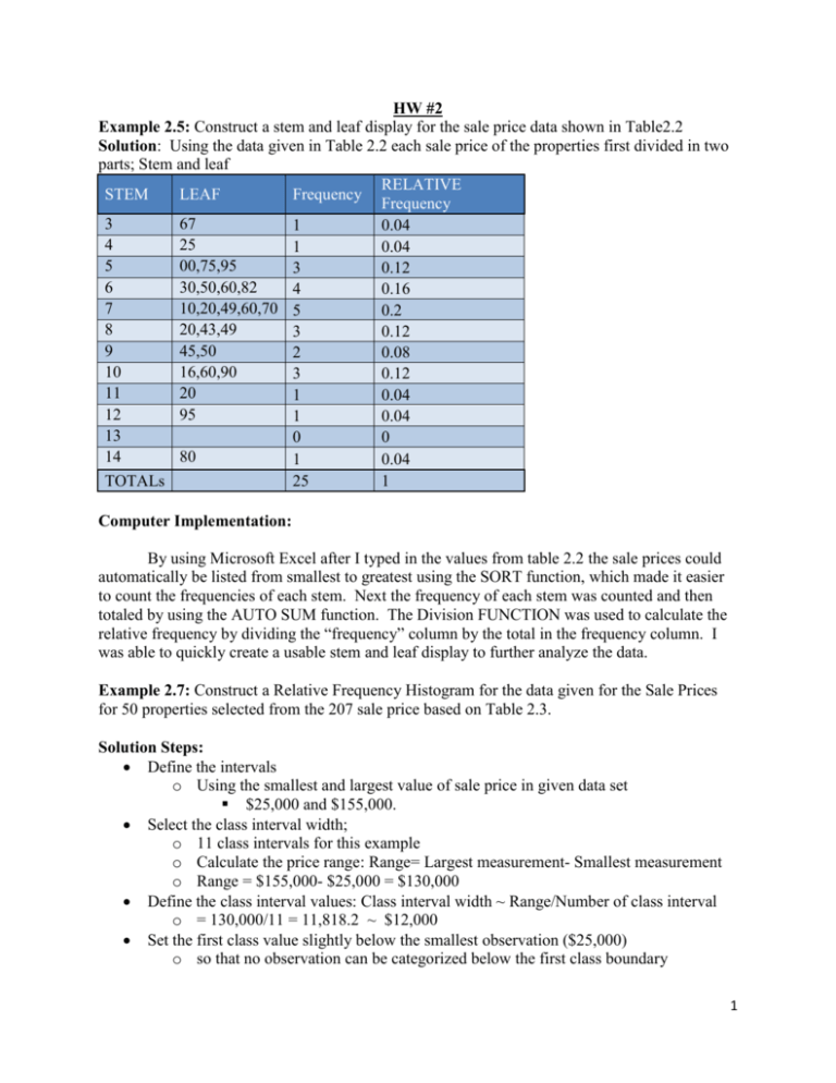
HW #2
Example 2.5: Construct a stem and leaf display for the sale price data shown in Table2.2
Solution: Using the data given in Table 2.2 each sale price of the properties first divided in two
parts; Stem and leaf
RELATIVE
STEM
LEAF
Frequency
Frequency
3
67
1
0.04
4
25
1
0.04
5
00,75,95
3
0.12
6
30,50,60,82
4
0.16
7
10,20,49,60,70 5
0.2
8
20,43,49
3
0.12
9
45,50
2
0.08
10
16,60,90
3
0.12
11
20
1
0.04
12
95
1
0.04
13
0
0
14
80
1
0.04
TOTALs
25
1
Computer Implementation:
By using Microsoft Excel after I typed in the values from table 2.2 the sale prices could
automatically be listed from smallest to greatest using the SORT function, which made it easier
to count the frequencies of each stem. Next the frequency of each stem was counted and then
totaled by using the AUTO SUM function. The Division FUNCTION was used to calculate the
relative frequency by dividing the “frequency” column by the total in the frequency column. I
was able to quickly create a usable stem and leaf display to further analyze the data.
Example 2.7: Construct a Relative Frequency Histogram for the data given for the Sale Prices
for 50 properties selected from the 207 sale price based on Table 2.3.
Solution Steps:
 Define the intervals
o Using the smallest and largest value of sale price in given data set
 $25,000 and $155,000.
 Select the class interval width;
o 11 class intervals for this example
o Calculate the price range: Range= Largest measurement- Smallest measurement
o Range = $155,000- $25,000 = $130,000
 Define the class interval values: Class interval width ~ Range/Number of class interval
o = 130,000/11 = 11,818.2 ~ $12,000
 Set the first class value slightly below the smallest observation ($25,000)
o so that no observation can be categorized below the first class boundary
1


Build the histogram using the class frequency
o Class Relative Frequency = Class Frequency / Total # of Observations
 = Class Frequency/50
Create the Histogram graph using Excel
Computer Implementation:
In Excel the above steps can be followed to back up the numbers that were found manually to
solve the problem. First, the descriptive statistics of the data was used to find the minimum,
max, range, and total number prices. Then the class intervals and values were determined
(manually). I plugged said values in to the histogram function in Excel and the below chart and
graph came up. The headings for the chart and graph needed to be modified slightly.
Sale Prices
Mean
66992.00
Standard Error
4063.07
Median
60750.00
Mode
25000.00
Standard Deviation
28730.21
Sample Variance
825425240.82
Kurtosis
1.13
Skewness
1.11
Range
130000.00
Minimum
25000.00
Maximum
155000.00
Sum
3349600.00
Count
50.00
Class
Frequency
36050
4
48050
10
60050
11
72050
8
84050
6
96050
3
108050
2
120050
3
132050
1
144050
1
156050
1
More
50
Relative
frequency
8.00%
28.00%
50.00%
66.00%
78.00%
84.00%
88.00%
94.00%
96.00%
98.00%
100.00%
100.00%
2
Example 3.1: Find the value of ∑x for the recorded observation are 2, 1, 3,2,3
Solution: The ∑ explain us the sum of values in the data set, therefore,
∑x = 2+1+3+2+3 = 11
Find the value of ∑x2 explain us to sum the square of the x-values in the data set, there fore
∑x2 = (2)2+ (1)2+(3)2+(2)2+(3)2= 4+1+9+4+9= 27
Computer Implementation:
Using Excel the autosum button can be used to find the sum of all data entered. The data can
also be squared using another function of Excel
Example 3.2: Refer to example 3.1
Find ∑(x-3) it explain us subtract 3 from each x and then sum all x value
∑(x-3) = (2-3)+ (1-3)+(3-3)+(2-3)+(3-3)= -1-2+0-1+0= -4
Find ∑(x-3)2 it explain us subtract 3 from each x value in the data set, square the differences and
then add each value to get the solution
∑(x-3)2= (2-3)2+ (1-3)2+(3-3)2+(2-3)2+(3-3)2= (-1)2+(-2)2+(0)2+(-1)2+(0)2= 1+4+0+1+0= 6
Find ∑x2-3 explain us to fisrt sum the square of each value of x then subtract 3 from the sum,
therefore,
∑x2-3= (2)2+ (1)2+(3)2+(2)2+(3)2-3 = 4+1+9+4+9-3= 24
Computer Implementation:
By typing the functions in one cell of Excel the function(s) can be copied to some or all data.
Example 3.8: Find the variance for the sample measurements 3, 7, 2, 1, 8
The variance S2 of a set of n samples measurement is equal to the sum of square of deviations of
the measurement about their mean divided by the value of (n-1) - S2 = ∑(x- x )2/(n-1)
Solution:
x= ∑x/n = (3+7+2+1+8)/5 = 21/5 = 4.2
The value of (x- x )2 is calculated in following table using Excel
Observations (x) x- xbar (x- xbar )2
sample variance:
3
-1.2
1.44 The
2
S
=
∑(x- x )2/n-1 = 38.8/4 = 9.7
7
2.8
7.84
2
-2.2
4.84
1
-3.2
10.24
8
3.8
14.44
TOTALs
21
0
38.8
Computer Implementation: All above computations were completed in Excel
3
Example 3.14: Calculating the z- score provided value of sale price (x), mean( x ) and standard
deviation (s) are Given: x= $200,000; x = $106,405 and s= $85,414
Solution Steps:
 Calculate z-score: z = (x- x )/ s
o z = (200,000-106,405)/ 85,414 = 1.10
 Analyze the z-score
o Because the z-score value is positive it can be determined $200,000 sale price is
1.10 standard deviation to the right of the mean $106,405
Computer Implementation:
Excel could be used to compute the z score, but a calculator is just as efficient.
4