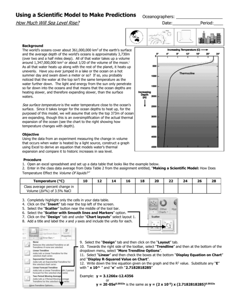
Using a Scientific Model to Make Predictions
How Much Will Sea Level Rise?
Oceanographers: ____________________
Date:____________Period:____
Background
The world’s oceans cover about 361,000,000 km2 of the earth’s surface
and the average depth of the world’s oceans is approximately 3,730m
(over two and a half miles deep). All of that water takes up a volume
around 1,347,000,000 km3 or about 1/20 of the volume of the moon.i
As all that water heats up along with the rest of the planet, it heats up
unevenly. Have you ever jumped in a lake or the ocean on a hot
summer day and swam down a meter or so? If so, you probably
noticed that the water at the top isn’t the same temperature as the
water further down. The light and energy from the sun only penetrate
so far down into the oceans and that means that the ocean depths are
heating slower, and therefore expanding slower, than the surface
waters.
Sea surface temperature is the water temperature close to the ocean's
surface. Since it takes longer for the ocean depths to heat up, for the
purposed of this model, we will assume that only the top 373m of ocean
are expanding, though this is an oversimplification of the actual thermal
expansion of the ocean (see the chart to the right showing how
temperature changes with depth).
Objective
Using the data from an experiment measuring the change in volume
that occurs when water is heated by a light source, construct a graph
using Excel to derive an equation that models water’s thermal
expansion and compare it to historic increases in sea level.
Procedure
1. Open an excel spreadsheet and set up a data table that looks like the example below.
2. Enter in the class data average from Data Table 2 from the assignment entitled, “Making a Scientific Model: How Does
Temperature Effect the Volume Of liquids?”
Temperature (°C)
10
12
14
16
18
20
22
24
26
28
Class average percent change in
Volume (ΔV%) of 3.5% NaCl
3.
4.
5.
6.
7.
8.
Completely highlight only the cells in your data table.
Click on the “Insert” tab near the top left of the screen.
Select the “Scatter” button near the middle of the tool bar.
Select the “Scatter with Smooth lines and Markers” option.
Click on the “Design” tab and under “Chart layouts” select layout 1.
Add a title and label the x and y axes and include the units for each.
9. Select the “Design” tab and then click on the “Layout” tab.
10. Towards the right side of the toolbar, select “Trendline” and then at the bottom of the
dropdown menu, select “More Trendline Options”.
11. Select “Linear” and then check the boxes at the bottom “Display Equation on Chart”
and “Display R-Squared Value on Chart”.
12. Write down the line equation given on the graph and the R2 value. Substitute any “E”
with “ x 10^ ” and “e” with “2.7182818285”
Example: y = 3.1266x-12.4356
or
y = 2E-05e0.5933x is the same as y = (2 x 10-5) x (2.7182818285)0.5933x
Equation: _______________________________________ R2 = ______________________
Analysis
The equation of the line given represents the “best fit line” for the data observed. It helps us model how the volume of water will
respond at temperatures where we didn’t collect data. Use your equation to check to see how accurate our model is. Pick a
temperature value that we did measure, i.e. 10˚, 12˚, 14˚, etc. and use that as the x-value in the equation. The y-value given
from this calculation is a statistical approximation of the actual measured percent change in volume of the water. The equation
is given an R2 value which indicated how good of a fit the modeled line is for the actual data points collected. R 2 values are
between 0 and 1. The closer to 1 the R2 value is, the better the modeled line fits the actual data. Usually scientists prefer R2
values to be between 0.9 and 1 because they demonstrate a statistically strong fit and mean that the model is a useful predictor.
1. Pick an x-value (10-28˚C) that you collected data for and use it in the equation you derived from Excel to find what y-value is
predicted by the model. Show your work below and put your answer in the box provided. Round your answer to the nearest
100th.
y=
2. How does your answer from the previous question compare with the class average percent change in volume measured at the
same temperature? How well did the model predict the observed y-value? What does the R2 value given tell you about how
confident you should be in your model?
3. Pick an x-value between 0-40˚C that wasn’t measured and use the equation to predict the percent change in volume that
would be observed at that temperature. Show your work below and put your answer in the box provided. Round your answer to
the nearest 100th.
y=
4. The rate at which sea water expands as temperature increases can be used to predict how much sea level will rise due to
thermal expansion. Because the surface area of the world’s oceans is so great, as the water expands, the change in the surface
area is less than 2.5%. Therefore, for our prediction of sea level rise, we will assume that the surface area of the ocean is
constant.
Given:
Initial Sea surface depth = 373m = Di
Initial Ocean surface area = 361,000,000 km2 = SAi
Sea surface volume = (SAi)(Di) = Vi
Percent Change in volume at 11˚C from experimental model = ΔV% (use the equation from Excel to find this value)
Sea level rise = change in depth = ΔD
Calculate: Using the known volume of the oceans and the rate of thermal expansion from our experiment, we can calculate the
change in volume of the oceans using the equation (ΔV) = (Vi)(ΔV%)
Since (SAi)(Di) = Vi, the equation above can be written as (ΔSA)(ΔD) = (SAi)(Di)(ΔV%)
As stated above, it can be assumed that the SA is the same before and after the ocean’s thermal expansion. Therefore the
equation can be simplified to the one below with only adding 2.5% error to our prediction of sea level rise. Use the equation
below to predict sea level rise given a 1˚C rise in global average sea surface temperature from 10˚C to 11˚C. Show your work
below and put your answer in the box provided. Round your answer to the nearest 100th.
(ΔD) = (Di)(ΔV%)
http://www.nodc.noaa.gov/dsdt/cwtg/spac.html
ΔD =
i
"The World Ocean." The Columbia Encyclopedia. CD-ROM. 2007, 6th Ed. New York: Columbia University Press.