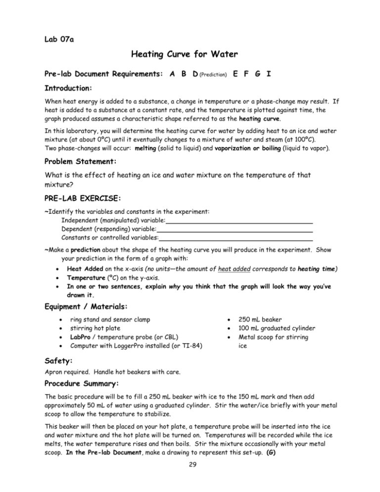
Lab 07a
Heating Curve for Water
Pre-lab Document Requirements: A B D (Prediction) E F G I
Introduction:
When heat energy is added to a substance, a change in temperature or a phase-change may result. If
heat is added to a substance at a constant rate, and the temperature is plotted against time, the
graph produced assumes a characteristic shape referred to as the heating curve.
In this laboratory, you will determine the heating curve for water by adding heat to an ice and water
mixture (at about 0ºC) until it eventually changes to a mixture of water and steam (at 100ºC).
Two phase-changes will occur: melting (solid to liquid) and vaporization or boiling (liquid to vapor).
Problem Statement:
What is the effect of heating an ice and water mixture on the temperature of that
mixture?
PRE-LAB EXERCISE:
~Identify the variables and constants in the experiment:
Independent (manipulated) variable:
Dependent (responding) variable:
Constants or controlled variables:
~Make a prediction about the shape of the heating curve you will produce in the experiment. Show
your prediction in the form of a graph with:
Heat Added on the x-axis (no units—the amount of heat added corresponds to heating time)
Temperature (ºC) on the y-axis.
In one or two sentences, explain why you think that the graph will look the way you’ve
drawn it.



Equipment / Materials:




ring stand and sensor clamp
stirring hot plate
LabPro / temperature probe (or CBL)
Computer with LoggerPro installed (or TI-84)



250 mL beaker
100 mL graduated cylinder
Metal scoop for stirring
ice
Safety:
Apron required. Handle hot beakers with care.
Procedure Summary:
The basic procedure will be to fill a 250 mL beaker with ice to the 150 mL mark and then add
approximately 50 mL of water using a graduated cylinder. Stir the water/ice briefly with your metal
scoop to allow the temperature to stabilize.
This beaker will then be placed on your hot plate, a temperature probe will be inserted into the ice
and water mixture and the hot plate will be turned on. Temperatures will be recorded while the ice
melts, the water temperature rises and then boils. Stir the mixture occasionally with your metal
scoop. In the Pre-lab Document, make a drawing to represent this set-up. (G)
29
Data Collection:
In the Pre-lab Document, prepare a proper data table for recording nine time and temperature data
points from your computer (or calculator). The title of the data table should be:
“Effect if Heat Added Over Time on a Mixture of Ice and Water”
Be sure to use proper column headings. Time will be measured in seconds. Temperature will be
measured in oC. The LoggerPro program will show both a list of the data points and a graph of the
data during the experiment.
In the Detailed Procedure, below, you will receive additional instructions concerning the use of
LoggerPro and which nine data points to record in your table.
Detailed Procedure:
A. Set up hot plate, ring stand, temperature probe and sensor clamp. Tape the cord of the
temperature probe to the thumbscrew of the sensor clamp. BEWARE – Do not let the cord touch
the hot plate. DO NOT turn on your hotplate yet.
B. USE the LOGGERPRO program on your computer WITH THE LABPRO MODULE:
LOGGERPRO Instructions
1.
Connect the green LabPro module to the computer using the USB cable.
Connect the power supply and listen for the “chirp”.
2.
Connect temperature probe to LabPro in CH1.
3.
Start the LoggerPro program on your computer by clicking on the
desktop icon.
4.
Click on “Experiment” and then “Data Collection” in the pull-down menu.
5.
OR, you can also click on
the “Data Collection” icon:
6.
When the
window opens you will
change several
“Data Collection”
need to check or
settings
7. Mode must be <Time Based>
8. Set the Length to <1000 sec>
9. Set Sampling Rate to <5>
(this is the right-hand box)
10. Click <Done> in the Data
11. DO NOT BEGIN
DATA.
seconds/sample
Collection window.
COLLECTING
C. Fill a 250 mL beaker with ice to the 150 mL mark and then add approximately 50 mL of water
using a graduated cylinder. Stir the water/ice briefly with your metal scoop to allow the
temperature to stabilize. Carefully drop the magnetic stirring bar into the beaker.
D. Place the beaker on the hot plate and put the temperature probe in the middle of the liquid,
making sure it does not touch the bottom, stirring bar or the sides of the beaker.
E. Turn on the stirring function of the hot plate and set it to about #3-4.
30
F. Turn on the hot plate to a high heat setting (about #7-9). Then, to begin collecting data, you
must go to:
LOGGERPRO  click/press the < GREEN ARROW> to begin collecting data
G. When the program has finished collecting data, go to:
LOGGERPRO  On the computer screen you will see a graph of the data. Along the left side
of the screen you will see the table of all the collected data in two columns: Time
(sec) and Temperature (oC). (The graph will have time on the x-axis and temperature
on the y-axis).
H. Data Collection: Click on the “Examine” button:
select the desired information.
Move the cursor using the mouse to
Record nine data points in the data table you made for your Pre-lab Document.
Select the data points at the beginning, middle, and end of the 1st plateau, 3 evenly spaced points
along the slope, and data points at the beginning, middle, and end of the second plateau.
Allow water in beaker to cool off and then empty beaker into the sink.
Data Analysis:

Plot a graph of temperature versus time with “Temperature” on the vertical axis and “Time”
on the horizontal axis. “Time” represents Heat because, as more time passed, more heat was
added. Be sure to use a straight edge to draw your graph, label the axes properly, and include
a title for your graph. Connect the points on your graph.

On the graph, label the following areas:
a.
b.
c.
d.

melting (ice + water)
water only
boiling (water + steam)
Label your graph sections with the correct heat formula (Q =) for each section.
See “Further Information” below.
Using a dashed line, extend the graph (extrapolate) as you believe it would appear if you
continued to heat the beaker until all the water boiled away and you were to record the
temperature of the steam. (You may have to research heating curves in your textbook!)
Further Information:
Pure water can be either solid or liquid at 0ºC. The temperature of a substance remains constant
when the liquid freezes or the solid melts. The temperature does not change until the phase change
is completed. The phase change energy is absorbed in melting or released in freezing. The energy
absorbed or released during the solid-liquid change of state is called the heat of fusion (Hf).
If we have pure water at a temperature of 0ºC, the temperature of the water will rise as heat is
added to the water. Eventually, the temperature of the water will reach 100ºC.
At 100ºC, pure water can be either liquid or gas. The temperature remains constant when the liquid
vaporizes or the gas condenses and doesn’t change until the phase change is completed. The energy
absorbed in vaporization and released in condensation is called the heat of vaporization (Hv).
The amount of heat absorbed during the different processes that occurred in the lab can be
calculated using the following formulae;
Heat absorbed during solid-liquid phase change (melting): Q = mHf
Heat absorbed by water during warming: Q = mcT
Heat absorbed during liquid-gas phase change (vaporization): Q = mHv
Total Heat Absorbed (Q) = mHf + mcT + mHv
31
Written Summary:
Discuss your experimental results in paragraph form (several paragraphs!). Include the following:
 Begin by evaluating your Prediction (Hypothesis). Do your results (the graph you made from
your data) agree with your prediction (the graph you made for your Pre-lab Document)? If
not, can you offer an explanation as to why that might be?
 Give a basic description of the heating curve for water based on the graph of your data.
 What is the melting temperature of ice, according to your graph
 What is the boiling temperature of water, according to your graph.
 Suggest reasons for why the melting temperature, according to your data, might not be
exactly 0ºC and why the boiling temperature might not be exactly 100ºC.
 Describe the energy changes (potential energy and kinetic energy) in the experiment and how
they relate to temperature changes.
You may use the graph paper on the next page for your final graph. You should use the graph paper in
the “Portrait Orientation” for your graph. Please review the Graphing Requirements in the front
section of your Laboratory Manual.
32
32a
IF YOU ARE USING A LABPRO WITH A TI-84 / TI NSPIRE CALCULATOR, FOLLOW THESE
EXTRA INSTRUCTIONS
LabPro Instructions
1.
Plug the Temperature Probe into Channel 1 of the LabPro. Use the link cable to
connect the TI Graphing Calculator to the LabPro. Firmly press in the cable ends.
2. Turn on the calculator and start the DATAMATE program (or application if you have a
TI-83+). Press CLEAR to reset the program.
3. Set up the calculator and interface for the Temperature Probe.
a. Select SETUP from the main screen.
b. If the calculator displays a Temperature Probe in CH 1, proceed directly to Step 4.
If it does not, continue with this step to set up your sensor manually.
c. Press
ENTER
to select CH 1.
d. Select TEMPERATURE from the SELECT SENSOR menu.
e. Select the Temperature Probe you are using (in °C) from the TEMPERATURE menu.
4. Set up the data-collection mode.
a. To select MODE, press
once and press
ENTER
.
b. Select TIME GRAPH from the SELECT MODE menu.
c. Select CHANGE TIME SETTINGS from the TIME GRAPH SETTINGS menu.
d. Enter “5” as the time between samples in seconds.
e. Enter “180” as the number of samples. The length of the data collection will be 15
minutes.
f. Select OK to return to the setup screen.
g. Select OK again to return to the main screen. Check the temperature reading in
the upper right corner and verify if it is reasonable.
h. DO NOT BEGIN COLLECTING DATA.
When you are ready to begin collecting data:
LabPro  select START to begin collecting data (you should hear four beeps)
When you are finished collecting data:
LabPro  On the calculator screen you will see a graph of the temperature data you
have collected (time on the x-axis and temperature on the y-axis).
When you are ready to record data points in your data table:
TI-84 / TI NSPIRE CALCULATOR  Move the cursor along the graph using the
arrows. Record data points at the beginning, middle, and end of the 1st plateau, 3
evenly spaced points along the slope, and data points at the beginning, middle, and end
of the second plateau.
32 b