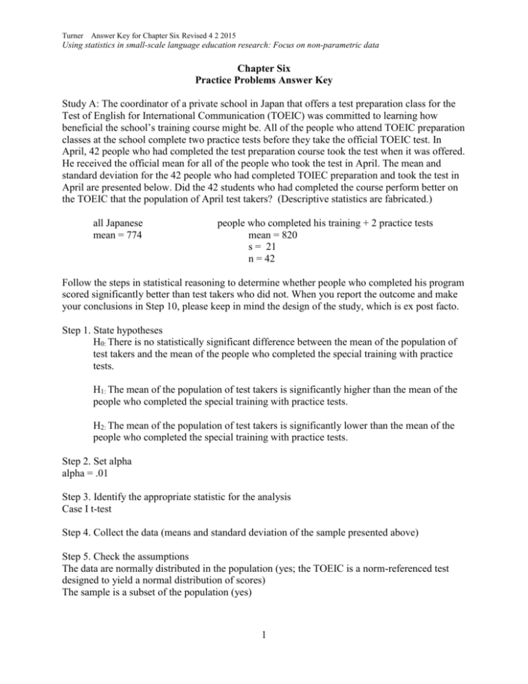
Turner
Answer Key for Chapter Six Revised 4 2 2015
Using statistics in small-scale language education research: Focus on non-parametric data
Chapter Six
Practice Problems Answer Key
Study A: The coordinator of a private school in Japan that offers a test preparation class for the
Test of English for International Communication (TOEIC) was committed to learning how
beneficial the school’s training course might be. All of the people who attend TOEIC preparation
classes at the school complete two practice tests before they take the official TOEIC test. In
April, 42 people who had completed the test preparation course took the test when it was offered.
He received the official mean for all of the people who took the test in April. The mean and
standard deviation for the 42 people who had completed TOIEC preparation and took the test in
April are presented below. Did the 42 students who had completed the course perform better on
the TOEIC that the population of April test takers? (Descriptive statistics are fabricated.)
all Japanese
mean = 774
people who completed his training + 2 practice tests
mean = 820
s = 21
n = 42
Follow the steps in statistical reasoning to determine whether people who completed his program
scored significantly better than test takers who did not. When you report the outcome and make
your conclusions in Step 10, please keep in mind the design of the study, which is ex post facto.
Step 1. State hypotheses
H0: There is no statistically significant difference between the mean of the population of
test takers and the mean of the people who completed the special training with practice
tests.
H1: The mean of the population of test takers is significantly higher than the mean of the
people who completed the special training with practice tests.
H2: The mean of the population of test takers is significantly lower than the mean of the
people who completed the special training with practice tests.
Step 2. Set alpha
alpha = .01
Step 3. Identify the appropriate statistic for the analysis
Case I t-test
Step 4. Collect the data (means and standard deviation of the sample presented above)
Step 5. Check the assumptions
The data are normally distributed in the population (yes; the TOEIC is a norm-referenced test
designed to yield a normal distribution of scores)
The sample is a subset of the population (yes)
1
Turner
Answer Key for Chapter Six Revised 4 2 2015
Using statistics in small-scale language education research: Focus on non-parametric data
Step 6. Calculate the observed value of the statistic
tobserved 
X 
s
x
nx

=
774  821
46
=
=
21/ 6.48
21/ 42
46
= -14.20
3.24
Step 7. use df and alpha to find the critical value of t.
df for Case I t-test is the number of people in the small group (the sample) minus one (nx – 1), so
df = 41. I used df = 40 in the chart of critical values on pp. 104-105, so tcritical = 2.7045.
Step 8. I compare the absolute value of tobserved to tcritical in this step.
I must remove the negative sign from the tobserved value.
14.20 is greater than 2.7045
So following the rules in statistical logic, I reject the null hypothesis. I accept the appropriate
alternative hypothesis (the one that states that the population mean is less than the mean of the
sample, H2, and make the probability statement).
Step 9. I can be 99% certain that the mean of the population of test takers is significantly lower
than the mean of the people who completed the special training with practice tests.
Step 10. I interpret meaningfulness in this step.
The researcher can be confident that the students who took the test preparation class performed
significantly better than the population of test takers (tobserved = 14.02, df = 41, alpha = .01), and
the difference is quite strong (effect size = .91); however, the research design is ex post facto, so
the findings do not support a causal statement. (That is, the researcher can be confident that there
is a statistically significant difference, but the researcher cannot assert that the difference is due
to the learners’ participation in the test preparation course!).
Effect size
t2
=
t 2  df
14.02 2
=
14.02 2  41
196.56
=
196.56  41
196.56
=
237.56
.83 = .91
Study B: A teacher wanted to know whether students would benefit from completing and
discussing a practice final test before taking the final test itself. She designed two equivalent
forms of her final test and distributed Form A to her students one week before the date of the
final exam so they could complete the practice test as homework. She reviewed the test with the
students during the class meeting two days before the final test date administration date. The
students completed Form B as the final exam. She compared the students’ scores on Form A to
the scores on Form B to determine whether there was a statistically significant difference in the
2
Turner
Answer Key for Chapter Six Revised 4 2 2015
Using statistics in small-scale language education research: Focus on non-parametric data
students' performance on the two test forms. Her students' scores on the Form A and Form B are
presented in the chart. Fill in the descriptive statistics and follow the steps in statistical logic to
determine whether the students performed differently on the two test administrations.
Student 1
Student 2
Student 3
Student 4
Student 5
Student 6
Student 7
Student 8
Student 9
Student 11
Student 11
Student 12
Student 13
mean
median
mode
standard
deviation
range
Score on A
69
70
75
76
76
78
78
80
81
81
90
89
80
Score on B
68
70
72
73
72
73
74
75
74
76
80
81
79
78.69
78
76, 78, 80, 81
6.101702
74.38
74
72, 73, 74
3.819652
21
13
Follow the steps in statistical reasoning to determine if there was a statistically significant
difference between participants’ performance on the two tests. When you report the outcome and
make your conclusions in Step 10, keep in mind the design of the study, which is preexperimental.
Step 1. State hypotheses
H0: There is no statistically significant difference between the mean of Test Form A and Test
Form B.
H1: There is a statistically significant positive difference between the mean of Test Form A
and Test Form B (the mean for Test Form A is significantly higher than the mean for Test
Form B).
H2: There is a statistically significant negative difference between the mean of Test Form A
and Test Form B (the mean for Test Form A is significantly lower than the mean for Test
Form B).
Step 2. Set alpha
alpha = .01
3
Turner
Answer Key for Chapter Six Revised 4 2 2015
Using statistics in small-scale language education research: Focus on non-parametric data
Step 3. Identify the appropriate statistic for the analysis
Case II Paired Samples t-test
Step 4. Collect the data (presented in chart with descriptive statistics, R commands below)
> scorea = c(69, 70, 75,76, 76, 78, 78, 80, 81, 81, 90, 89, 80)
> scoreb = c(68, 70, 72, 73, 72, 73, 74, 75, 74, 76, 80, 81, 79)
> summary (scorea)
Min. 1st Qu. Median Mean 3rd Qu. Max.
69.00 76.00 78.00
78.69 81.00 90.00
> sd (scorea)
[1] 6.101702
> subset(table(scorea), (table(scorea)==max(table(scorea))))
scorea
76 78 80 81
2 2 2 2
> 90-69
[1] 21
> summary(scoreb)
Min. 1st Qu. Median Mean 3rd Qu. Max.
68.00 72.00 74.00 74.38 76.00 81.00
> sd (scoreb)
[1] 3.819652
> 81-68
[1] 13
> subset(table(scoreb), (table(scoreb)==max(table(scoreb))))
scoreb
72 73 74
2 2 2
Step 5. Check the assumptions
Both sets of data are normally distributed. Review histograms and interpret Shapiro Wilk. (It
appears that I can be reasonably certain the data are normally distributed).
> hist (scorea, col = "light green")
> hist (scoreb, col = "light blue")
4
Turner
Answer Key for Chapter Six Revised 4 2 2015
Using statistics in small-scale language education research: Focus on non-parametric data
> shapiro.test(scorea)
Shapiro-Wilk normality test
data: scorea
W = 0.9334, p-value = 0.3767
> shapiro.test (scoreb)
Shapiro-Wilk normality test
data: scoreb
W = 0.9558, p-value = 0.6877
Step 6. Calculate the observed value of the statistic
I used R.
>t.test (scorea, scoreb, paired =T)
Paired t-test
data: scorea and scoreb
t = 5.4137, df = 12, p-value = 0.0001566
alternative hypothesis: true difference in means is not equal to 0
95 percent confidence interval:
2.574014 6.041370
sample estimates:
mean of the differences
4.307692
Step 7.
Using the critical value approach—
Determine tcritical using df and alpha
5
Turner
Answer Key for Chapter Six Revised 4 2 2015
Using statistics in small-scale language education research: Focus on non-parametric data
The formula for df for the Case II Paired Samples t-test (npairs – 1), so df = 13 – 1 =12.
The chart in Chapter Five on pp. 104-105 gives tcritical as 3.0545 (df = 12, α = .0.1)
Using the exact probability approach—
I simply retrieve the exact probability from the R output; exact p = 0.0001566.
Step 8.
Using the critical value approach—
Compare tobserved to tcritical
5.4137 is greater than 3.0545 so reject null hypothesis & accept appropriate alternative
Using the exact probability approach—
Compare exact probability to alpha
0.0001566 is less than alpha so reject null hypothesis & accept the appropriate alternative
Step 9. Make probability statement
I can be 99% certain that there is a statistically significant positive difference between the mean
of Test Form A and Test Form B (the mean for Test Form A is significantly higher than the
mean for Test Form B).
Step 10. Interpret meaningfulness
The teacher/researcher can be confident that students do better on the practice test than the
actual final, so she concludes that having her students complete and discuss a practice final test is
not beneficial (tobserved = 5.4137, df = 12, p <.01, effect size = .84). (Incidentally, I don’t agree
with her interpretation, but that’s what she thinks on the basis of this fabricated data!) .
Effect size
t2
=
t 2  df
5.4137 2
=
5.4137 2  12
29.3081
=
29.3081  12
29.3081
=
41.3081
.71 = .84
Study C: The researcher for a large school district is investigating whether 5th grade children
whose parents receive coaching in how to help their children with homework do better achieve a
greater degree of learning than children whose parents haven’t been coached. The researchers
randomly selected 80 5th grade children to participate in the study. The parents of 40 of the 5th
grade children, randomly selected from the 80 that had been randomly selected, were invited to
participate in 6 hours of coaching on how to help their children do homework assignments. After
these sessions, throughout the term, the parents participated in follow-up sessions during which
they received additional tips on how to help their children. The parents also turned in biweekly
surveys that helped the researcher verify that the parents had been following the advice they had
received. The parents of the other group of 40 children received the usual reports on their
children's progress in school. At the end of the term, all of the children took a state test intended
to measure students’ learning. The test is designed to yield normally distributed scores. The
6
Turner
Answer Key for Chapter Six Revised 4 2 2015
Using statistics in small-scale language education research: Focus on non-parametric data
researcher compared the performance of the children whose parents were coached to the
performance of children whose parents weren’t coached. The data are located in the resource
section of the companion website.
1. What is the independent variable and what are its levels?
+/- coaching for children’s parent
2. What is the dependent variable?
Students’ learning
3. Identify the major category of research design and your reasons for your choice.
There is a treatment (the innovation of coaching students’ parents in how to assist their children
with their homework). This research takes place in a large school district—so the design may be
true experimental. If the school district is not sufficiently large to be considered a population,
the design is pre-experimental.
Now follow the 10 steps in statistical logic to determine whether the children whose parents were
coached performed significantly better on the state test than the children whose parents weren't
coached.
The descriptive statistics for the two groups are presented below. The (fabricated) children's
scores on the state test were sent by email if you want to use R. (I did the calculations using R,
and followed the procedure described in Chapter Six for separating the coached from the
uncoached to determine the descriptive statistics for the two groups and check the assumptions.
See my R commands inserted in the steps below).
Parents Coached
mean = 85.25
s = 5.77
n = 40
Parents Un-coached
mean = 80.30
s = 7.85
n = 40
Step 1. State hypotheses
H0: There is no statistically significant difference in the learning of 5th graders whose parents
received coaching on helping with homework and those whose parents did not receive coaching.
H1: There is a statistically significant positive difference in the learning of 5th graders whose
parents received coaching on helping with homework and those whose parents did not receive
coaching.
H2: There is a statistically significant negative difference in the learning of 5th graders whose
parents received coaching on helping with homework and those whose parents did not receive
coaching.
Step 2. Set alpha
alpha = .01
Step 3. Identify the appropriate statistic for the analysis
Case II Independent Samples t-test
7
Turner
Answer Key for Chapter Six Revised 4 2 2015
Using statistics in small-scale language education research: Focus on non-parametric data
Step 4. Collect the data
I imported the data set using this command
>data.coaching.problem = read.csv(file.choose(), header =T)
I viewed the data set using this command:
> View (data.coaching.problem)
Here’s the dataset; the coached group is “1” and uncoached group is “2” (I think). All dependent
variable values for all of the participants are in one column (with the heading, score). This way
of formatting the spreadsheet is the approach typically used by researchers.
Student coached score
1
1
76
2
1
76
3
1
76
4
1
77
5
1
77
6
1
79
7
1
79
8
1
80
9
1
80
10
1
80
11
1
81
12
1
81
13
1
82
14
1
82
15
1
84
16
1
84
17
1
84
18
1
84
19
1
84
20
1
85
21
1
85
22
1
86
23
1
86
24
1
87
25
1
87
26
1
87
27
1
88
28
1
88
29
1
88
8
Turner
Answer Key for Chapter Six Revised 4 2 2015
Using statistics in small-scale language education research: Focus on non-parametric data
30
31
32
33
34
35
36
37
38
39
40
41
42
43
44
45
1
1
1
1
1
1
1
1
1
1
1
2
2
2
2
2
89
89
91
91
92
92
92
93
94
96
98
70
70
70
70
70
Step 5. Check the assumptions
The assumptions are:
 1) The independent variable is nominal and has only two levels.
 2) There are different participants in the two groups.
 3) The dependent variable is interval or interval-like.
 Make and interpret a histogram of each group’s data
 Calculate and interpret the Shapiro Wilk statistic for each group
 4) The groups are exactly the same size, or the variances (standard deviation
squared) of the groups are approximately equal.
 Verify that groups are same size OR
 Calculate the Levene Test statistic to verify that variances are
approximately equal OR
 Use R (and Welch’s formula, which corrects for violation) to calculate
tobserved .
I need to split the complete dataset to check assumptions 3 & 4 and calculate the descriptive
statistics (which are typically reported!). I follow the steps in Chapter Six, Box 6.1 to split the
complete dataset, making separate datasetfor the coached group and the uncoached group—and I
use the length command to see how many people are in each group (yes, each group has 40
participants).
> coached.data = subset (data.coaching.problem, data.coaching.problem$coached=="1") [Note
that I enter a name for the coached data (coached.data), then enter the subset command. The
name of the complete dataset is given next, then the name of the column in that dataset that
includes the independent variable values; I tell R to make a dataset called coached.data which
includes only the people who are in Group 1.]
9
Turner
Answer Key for Chapter Six Revised 4 2 2015
Using statistics in small-scale language education research: Focus on non-parametric data
> uncoached.data = subset (data.coaching.problem, data.coaching.problem$coached=="2")
[Now I make a dataset called uncoached.data]
> length (coached.data$score)
[1] 40
> length (uncoached.data$score)
[1] 40
> summary (coached.data$score)
Min. 1st Qu. Median Mean 3rd Qu. Max.
76.00 80.75 85.00
85.25 89.00 98.00
> sd (coached.data$score)
[1] 5.767949
> 98-76
[1] 22
> subset (table(coached.data$score),
(table(coached.data$score)==max(table(coached.data$score))))
84
5
> summary (uncoached.data$score)
Min. 1st Qu. Median Mean 3rd Qu. Max.
70.0 73.0 79.0
80.3 87.0
93.0
> sd (uncoached.data$score)
[1] 7.845299
> subset (table(uncoached.data$score),
(table(uncoached.data$score)==max(table(uncoached.data$score))))
70 73
5 5
> 93-70
[1] 23
Here are the descriptive statistics.
Coached (1)
mean
85.25
median
85
mode
84
Uncoached (2)
80.30
79
70, 73
10
Turner
Answer Key for Chapter Six Revised 4 2 2015
Using statistics in small-scale language education research: Focus on non-parametric data
standard deviation
range
5.767949
22
7.845299
23
I then made histograms and calculated the Shapiro Wilk statistic for each group.
>par (mfrow = c(1,2))
> hist (coached.data$score, col = "red")
> hist (uncoached.data$score, col = "purple")
> shapiro.test (coached.data$score)
Shapiro-Wilk normality test
data: coached.data$score
W = 0.9735, p-value = 0.4608
> shapiro.test(uncoached.data$score)
Shapiro-Wilk normality test
data: uncoached.data$score
W = 0.9093, p-value = 0.003602
11
Turner
Answer Key for Chapter Six Revised 4 2 2015
Using statistics in small-scale language education research: Focus on non-parametric data
The histogram and the Shapiro Wilk statistic indicate that the data for the uncoached group are
probably not normally distributed, so the Case II Independent Samples t-test SHOULD NOT be
used (the non-parametric Wilcoxon Rank Sum Test is appropriate instead), but I’ll go ahead and
calculate the Independent Samples t-test statistic, so we can see the outcome, and because the
details of the Wilcoxon statistics are presented in the next chapter!
I don’t need to calculate the Levene Test statistic because the groups are the same size (and
because R uses the Welch formula for calculating the Case II Independent Samples t-test which
corrects for any difference between the standard deviations of the two groups).
Step 6. Calculate tonserved.
There are several ways to enter the data for the t-test. I can do it using the two separate groups,
like this:
> t.test(coached.data$score, uncoached.data$score)
Or I can use the complete data set like this:
t.test (score ~ coached, data = data.coaching.problem) [Note that the name of the dependent
variable is first inside the parentheses; then a tilde and the name of the independent variable; then
data = and the name of the complete data set.]
Welch Two Sample t-test
data: score by coached
t = 3.2151, df = 71.628, p-value = 0.001957
alternative hypothesis: true difference in means is not equal to 0
95 percent confidence interval:
1.880539 8.019461
sample estimates:
mean in group 1 mean in group 2
Step 7.
Using the critical value approach—
Determine tcritical using df and alpha
The formula for df for the Case II Independent Samples t-test (n1 – 1) + (n2 -1), so df = 78
I used df = 70 from the chart in Chapter Five on pp. 104-105 so tcritical = 2.6479
Using the exact probability approach—
I simply retrieve the exact probability from the R output, so exact p = 0.001957.
Step 8.
Using the critical value approach—
Compare tobserved to tcritical
12
Turner
Answer Key for Chapter Six Revised 4 2 2015
Using statistics in small-scale language education research: Focus on non-parametric data
3.2151 is greater than 2.6479 so reject null hypothesis & accept the alternative, H1
Using the exact probability approach—
Compare exact probability to alpha
0.001957 is less than alpha so reject null hypothesis & accept the alternative, H1
Step 9. Make the appropriate probability statement
I can be 99% certain that there is a statistically significant positive difference in the learning of
5th graders whose parents received coaching on helping with homework and those whose parents
did not receive coaching.
Step 10. Interpret meaningfulness.
On the basis of these (fabricated) data, we can be confident that students whose parents are
coached on how to help their children with their homework achieve a higher level of learning
than students whose parents do not receive this coaching (tobserved = 3.2151, df = 71.628*, alpha <
.01). The effect size (.355) indicates that the difference is strong.
*Note that I used R to calculate the observed value of t, which used the Welch formula and
corrects for the difference in the variances of the two groups. This correction is reflected in the
degrees of freedom.
Effect size calculation:
t2
=
t 2  df
3.21512
10.3369
=
=
3.2151  71.628
10.3369  71.628
13
10.3369
=
81.9649
.126 = .355