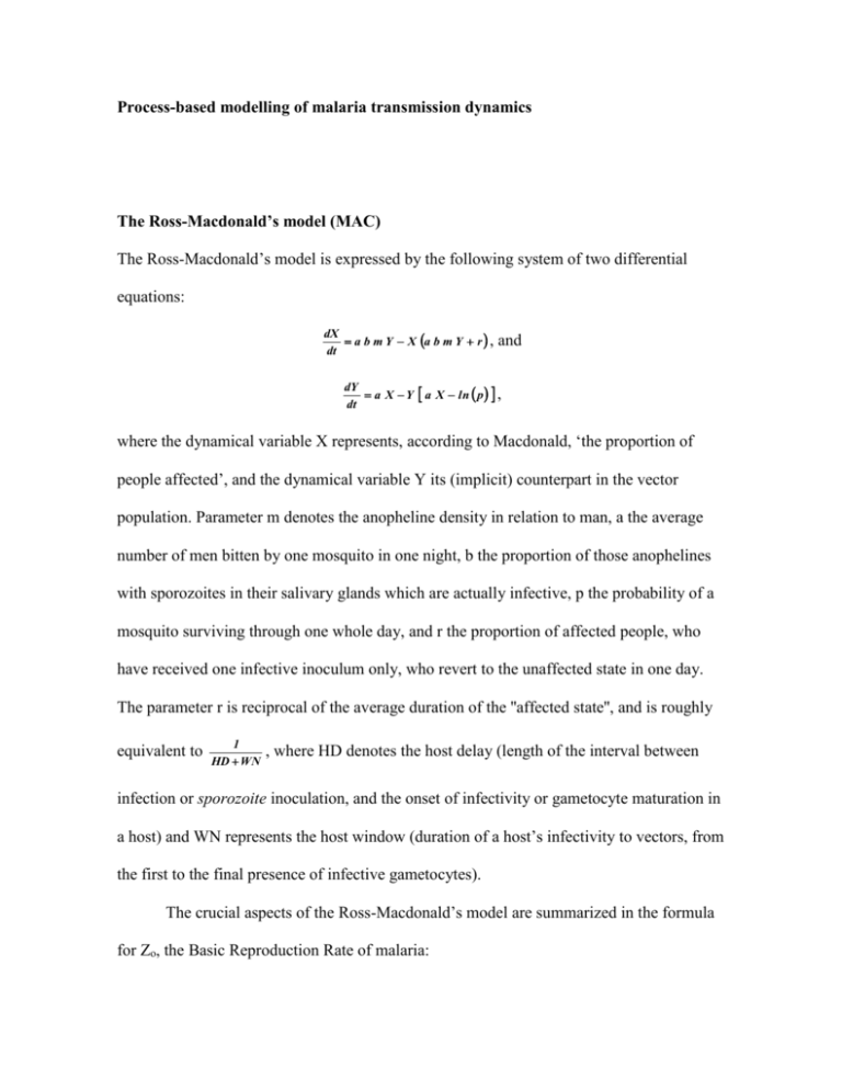
Process-based modelling of malaria transmission dynamics
The Ross-Macdonald’s model (MAC)
The Ross-Macdonald’s model is expressed by the following system of two differential
equations:
dX
 a b m Y  X a b m Y  r  ,
dt
and
dY
 a X  Y  a X  ln  p   ,
dt
where the dynamical variable X represents, according to Macdonald, ‘the proportion of
people affected’, and the dynamical variable Y its (implicit) counterpart in the vector
population. Parameter m denotes the anopheline density in relation to man, a the average
number of men bitten by one mosquito in one night, b the proportion of those anophelines
with sporozoites in their salivary glands which are actually infective, p the probability of a
mosquito surviving through one whole day, and r the proportion of affected people, who
have received one infective inoculum only, who revert to the unaffected state in one day.
The parameter r is reciprocal of the average duration of the ''affected state'', and is roughly
equivalent to
1
HD  WN
, where HD denotes the host delay (length of the interval between
infection or sporozoite inoculation, and the onset of infectivity or gametocyte maturation in
a host) and WN represents the host window (duration of a host’s infectivity to vectors, from
the first to the final presence of infective gametocytes).
The crucial aspects of the Ross-Macdonald’s model are summarized in the formula
for Zo, the Basic Reproduction Rate of malaria:
Z0 


 m a 2 b pn  b 
 C,
r  ln  p  
r
where the parameter n represents ‘the time taken for completion of the extrinsic cycle’, and:
C


 m a 2 pn
ln  p 
,
summarizes the ‘Vectorial Capacity’ of malaria.
Macdonald derived Zo as an estimate of the average number of secondary cases
arising in a very large population at risk of completely susceptible humans following the
introduction of a single primary case. Zo=1 was defined as the transmission threshold: for
values above, malaria cases will propagate; for values below, the disease will recede. The
formula for Zo holds that the influence of vector survivorship (p) is greater than the
influence of the average number of men bitten by one mosquito in one day (a) or the
sporogonic cycle (n), which are in turn greater than the influence of the proportion b, the
density m, or the proportion r. Hence, Macdonald considered the vector survivorship as the
single most important element in the Basic Reproduction Rate of malaria.
Macdonald’s affected proportions do not distinguish between infected and
infectious stages. His conclusion with respect to host infectivity was: ‘transmission can be
altered by reduction of the mean period of infectivity of a case of malaria. The influence is,
however, relatively low; the reproduction rate varies directly with the mean duration of
infectivity, very great changes in which would be necessary to reduce the high rates
common in Africa and some other places below the critical level’. Macdonald’s b is a
measure of incidence (e.g. by its role in expressions for ‘inoculation rate’ and ‘force of
infection’), and r the reciprocal of the average duration of the ‘affected’ state. Macdonald
wrote that ‘in nature, the value of the reproduction rate is greatly influenced by immunity
altering the values of r and b’.
The stock-flow model of the Ross-Macdonald’s model is shown in Figure 1.
The Anderson and May’s model (AM)
Anderson and May extended the Ross-Macdonald’s model by considering the proportions
of exposed individuals (Eh) and exposed mosquitoes (Em), and by including the latency of
infection in human hosts (th) and mosquito vectors (tm). The AM model is thus based on the
following system of four coupled ordinary differential equations (note time lags in the
equations):
dEh
 a b m Im t   1  Eh t   Ih t    a b m Im t  t h   1  Eh t  t h   Ih t  t h   e r  1 t h  r Ih t   1 Eh t  ,
dt
dIh
 a b m Im t  t h   1  Eh t  t h   Ih t  t h   e r  1 t h  r Ih t   1 Ih t  ,
dt
dEm
 a c Ih t   1  Em t   Im t    a c Ih t  tm   1  Em t  t m   Im t  t m   e  2 t m  2 Em t  ,
dt
and
dIm
 a c Ih t  tm   1  Em t  tm   Im t  tm   e  1 t m  2 Im t  .
dt
Variable a denotes the mosquito biting rate. Variable m, or mosquito density, is
calculated through the linear regression
m
3 R
d
, where 3 represents the rainfall to
mosquito constant, R the total monthly rainfall, and d the total human population at risk.
Lastly, parameters 1 and 2 represent, respectively, the mortality rates of humans and
mosquitoes. 2 is given by
2   log p  ,
mosquito vector, is expressed as
1 / U
where p, the daily survival probability of the
, and U denotes the total gonotrophic cycle length.
The mathematical model proposed by Worrall, Connor and Thomson (WCT)
This temperature- and rainfall-driven dynamic model of malaria transmission was proposed
to predict epidemics in areas where brief seasonal transmission and occasional epidemics
do not enable acquired immunity, and to examine the relationship between the intervention
timing and transmission intensity on the effectiveness of indoor residual spraying (IRS).
WCT is composed of six sub-models that allow estimating:
 (SM1) the number of adult female mosquitoes as a function of rainfall,
 (SM2) the length of the gonotrophic or feeding cycle as a function of
temperature,
 (SM3) the duration of the sporogonic cycle as a function of temperature,
 (SM4) the vector survivorship in terms of survival probability per
gonotrophic cycle and per day,
 (SM5) the sporozoite rate, and
 (SM6) the number of new infections, super-infections and recoveries.
The combination of SM3 and SM4 allows calculating ‘the probability of the vector
surviving long enough for sporogonic development to be completed’. SM4 is also used ‘to
simulate the effects of a residual spray program, which is considered in terms of its impact
upon the probability of vector survival per gonotrophic cycle’.
In SM1, the number of mosquitoes emerging each month (q) is estimated through
the linear regression
q R,
where  represents the linear scaling factor (or rainfall to
mosquito constant) and R the monthly rainfall total. In SM2, the total gonotrophic cycle
length (U) is estimated as:


fu
,
U    



T

l

g
u

where
fu
T  l   gu
(or u) represents the period of time required by a female Anopheles to
digest the blood meal (maturation of the ovaries), and  denotes the length of the period
required by the adult mosquito to search for a suitable water body, lay the cohort of eggs,
find a new host and bite again. fu represents the total number of degree-days needed to
complete development, gu the threshold temperature below which development ceases, and
(T+l) the indoor temperatures, which are function of the outdoor ambient temperatures (T)
and an adjustment factor (l). In SM3, the length of the sporogonic cycle is expressed as:
N
fN
( T N gN )
,
where fN represents the number of degree-days needed to complete development, and gN
denotes the temperature threshold below which development ceases. Temperature TN is
‘adjusted to account for differences between indoor and outdoor resting temperatures, using
a weighting system, based on the period of time the vector spends indoors as a proportion
of gonotrophic cycle length’,
TN  T 
lu
U
.
SM4 defines two populations of mosquitoes: covered (C) and not covered (1-C) by
the spray program, where C represents the percentage coverage achieved by the spraying
campaign. The daily survival probability of the mosquito vector is expressed as
1 / U
,
where  denotes the probability of the vector surviving each gonotrophic cycle (assumed to
be constant) in the population not covered by the campaign.  is reduced by  in the
population covered by the spray program immediately after spraying, gradually increasing
back towards  at a rate of /6 per month over the effective residual life of the insecticide
(assumed to be 6 months). Thus, the mean probability of the daily survival (P) for the
whole mosquito population is given by:
 ( 1  C )    C  1U .
In SM5, the sporozoite rate (S) is estimated using the equation:
S
xhkvP N
,
1    xhkv 
where x denotes the proportion of humans that are infectious, h the proportion of human
blood fed mosquitoes, k the probability of the vector becoming infected per infectious
meal, and v the probability of the vector becoming infectious with the malaria parasite. The
formula uses the probability of surviving the gonotrophic cycle for an unsprayed population
(); in a sprayed situation this parameter is substituted for  ( 1  C )  C  .
Lastly, in SM6 the frequency at which mosquitoes feed on humans (a) is estimated
as h/U, and the number of infectious mosquitoes biting humans is calculated as the product
of the sporozoite rate (S), the number of mosquitoes (q), and the person biting habit (a).
The probability of a human receiving an infectious bite (R) is given by
1

1 1 
d

Sqa
, where
d denotes the total human population at risk. The number of people recovering at time t (ct)
is given by
c  I  Z  r ,
where I represents the number of infected humans, r the probability
of recovery of new infected humans after time t, and Z the number of super-infections (or
Z= R I). Thus, the number of infected humans at time t (It) is given by:
I t  I t  1  ct  Ft
,
where Ft denotes the number of people newly infected at time t or R(d-I). The total number
of reported infected humans at time t is given by: *It, where  denotes the proportion of
positive cases in the community reported to health facilities.
The schematic diagram of the WCT model and the stock-flow diagrams of its SM3
(estimation of the length of the sporogonic cycle) and SM6 (dynamics of new infections,
super-infections and recoveries) sub-models are depicted in Figure 2.
The coupled mosquito-human model of malaria proposed by Alonso, Bouma and
Pascual (ABP)
The ABP coupled mosquito-human model was implemented to assess the impacts of
increasing trends in local ambient temperatures on malaria transmission dynamics in a
highland region of East Africa. The model was run with and without temperature trends
over a three-decade simulation period in order to address how much of a change in the size
of epidemics could be attributed to the observed warmer temperatures. The model couples
the dynamics of the disease in two main components: the human population and the
mosquito vector. The former consists of a classical system of ordinary differential
equations in which five different classes are considered: susceptible non-infected human
hosts (S), infected but non-infectious individuals (E), infected individuals who acquire
asymptomatic infection but are nevertheless infectious and can transmit malaria parasites to
mosquito vectors (I), recovered individuals/acquired immunity or those human hosts who
have cleared parasitaemia, or have too low a level of parasitaemia to effectively infect the
vector (R), and infected individuals who present symptoms and therefore receive some sort
of clinical treatment (C). The system of ordinary differential equations for this component
is given by:
dS
 B   S   R  H S   C
dt
,
dE
  S  H E   E
dt
,
dI
 1     E    I   C  r I   I   H I
dt
dR
 r I   R  H R
dt
,
, and
dC
   E    I   C   C   C  H C .
dt
In the formulation of the full version of the ABP model, the authors do not include
the parameters  and  in the dynamics of the total number of infected individuals who
acquire asymptomatic infection (I) and the total number of infected individuals who present
symptoms and therefore receive clinical treatment (C), respectively. Thus, the right-hand
side of their equations only includes five terms.
Exogenous variables B and H in the system of equations for the human host
component represent, respectively, the replenishment of susceptible individuals through
immigration or birth, and the individual losses due to mortality or more generally,
population turnover. In the model, variables B and H balance each other so that the total
human population at risk (N=S+E+I+R+C) remains constant. Thus, B=HN.
The transmission rate, , or “force of infection”, or the per-capita probability that
susceptible individuals acquire the infection per unit time as a result of infecting bites from
mosquitoes, is given by:
 b
M t 
 t  a  e ,
N
where b is the probability that an infectious bite results in infection, M(t) the total
population of mosquitoes, (t) the fraction of infectious mosquitoes at time t, and a the
number of bites per individual mosquito per unit time. The first term in  represents the
local transmission where the fraction of infectious mosquitoes at time t is a consequence of
acquiring the parasite from infectious humans at some earlier time. The second, additive
term e is an external force of infection and represents, for example, those individuals who
acquire malaria infection when visiting endemic areas.
The variable  represents the rate of loss of immunity and is a function of the
intensity of mosquito exposure (as the frequency of mosquito bites increases, the rate of
loss of immunity tends to decrease) as follows:
   

 
exp 
 0

 1


,
where  denotes the rate of infectious bites per human, which is given by

aW
N
, and 0
the loss of immunity basal rate, i.e. when  tends to zero. The variable W represents the
total number of infectious mosquitoes. The variable  represents the CS clearance or
recovery rate. The variable r represents the IR clearance or recovery rate and is a
function of the intensity of mosquito exposure (as the frequency of mosquito bites
increases, the recovery rate tends to decrease) as follows:
r   


exp 
 r0

 1


,
where r0 denotes the IR recovery basal rate, i.e. when  tends to zero.
1

denotes the average time in the exposed phase.  represents the fraction of
infections in humans that fully develops severe malaria symptoms and, then, receive
clinical treatment (C).  denotes a factor that decreases the per-capita transmission rate ()
when asymptomatic but infectious individuals (I) can present a relapse of severe malaria
symptoms if they are bitten again. Lastly, variable  represents the CI recovery rate.
Figure 3 depicts the stock-flow model of the human host component of the ABP
coupled mosquito-human model. The mosquito population model considers, in turn, the
number of larvae (L) and adult mosquitoes (M); see Figure 4. The dynamics of the level
variable L is given by:
dL
K L
f M
   L L  dL L ,
dt
 K 
where f is the per-capita fecundity rate or the maximum number of eggs that enter the larval
stage per female per unit time. Since female mosquitoes lay eggs only once between blood
meals, the fecundity and biting rates can be related following f = F a, where F denotes the
mosquito fecundity factor.
The number of eggs per adult female and unit time can be written as:
Nf  n a
, where
n is the number of eggs per oviposition event. The per-capita fecundity rate, f, should be
lower than Nf to account for some mortality at the egg stage.
The variable K denotes the larvae carrying capacity and is determined by rainfall,
since water pools of different size provide the habitat for mosquito breeding and larvae
development. Also, larvae survival decreases when precipitation is large, above a given
threshold that depends on how much rain has fallen in previous months. The carrying
capacity is modelled in ABP following:
dK
 k A P  kE K ,
dt
where kA and kE represent, respectively, the carrying capacity conversion factor and loss
rate. Variable L denotes the larval mortality rate and is approximated as follows:
 L  0   L T    L P  ,
where 0 is a basic mortality rate caused by temperature- or rain-independent processes,
such as predation. The temperature-dependent larval mortality rate, L(T), is given by:
1.1946  0.0804 T





14

1
/ 2  L 16    L 14 T  14 

 L T    L

1
/
3

L 16    L 18    L 20 



0
.
062157
 0.0052243 T

T  14 

14  T  16 

16  T  20 
20  T  34 
,
where L(14), L(16), L(18), and L(20) denote the per-capita larvae death rate (inverse of
the larval average life time) at temperatures of 14, 16, 18, and 20°C.
L(P) is a function that depends on daily rainfall and measures how much mortality
rate increases as a consequence of heavy rain. Specifically, L(P) is given by:

 L P    R  P  P 12
,
where R is a proportional factor transforming a positive deviation from the moving
average, due to a peak in rainfall, into an increase in larval mortality. This parameter, socalled death factor, is introduced to represent the washout effect for the larvae.  x  is x if x
> 0 and 0 otherwise. Lastly,
P 12
is a 12-month moving average calculated from the
rainfall time series.
Variable dL represents the larval development rate and is related to the ambient
temperature following a simple regression used for Anopheles gambiae:
d L  0.00554 T  0.06737
,
where T represents the temperature expressed in degrees Celsius.
The adult mosquito population is divided into three classes: susceptible non-infected
mosquitoes (X), infected non-infectious mosquitoes, or becoming exposed when they bite
an infectious human (V) and infectious mosquitoes (W). The system of ordinary differential
equations is given by:
dX
  c a y X   M X  dL L ,
dt
dV
  c a y X   P V  M V
dt
dW
  P V  M W
dt
, and
.
Variable c denotes the human host to mosquito probability of transmission.
Variables y and M represent, respectively, the fraction of human population transmitting
the parasite to the mosquito vector, and the adult mosquito mortality. The average lifetime
of mosquitoes depends on temperature as follows:
  4.4  1.31 T  0.03 T 2
.
Therefore, the per-capita death rate of adult mosquitoes can be written as:
M 
1

.
P is the per-capita rate at which new infectious mosquitoes arise, a quantity related to the
duration of sporogony. This development time is also influenced by temperature as follows:
 P  0.009 T  0.1441 ,
specifically for Plasmodium falciparum incubation within female mosquitoes.
The ABP model uses a simple regression between the inverse of the average
gonotrophic cycle (
1
ta
), or roughly the biting rate (expressed in number of bites per
mosquito per day), and the ambient temperature, as follows:
a~

1
 0.091678 T  1.7982 .
ta
In the ABP full model version the human E class and the mosquito V class for the
exposed individuals (not yet infectious) are divided into nH and nV latent classes (not shown
here), respectively. The means of these incubation times are given by 1/H and 1/V,
respectively, whereas their variances decrease as function of the number of latent classes.
The outdoor ambient temperature drives the larval parameters L and dL. The ABP
model also considers an effective temperature, Te, which is higher than the outdoor ambient
temperature, in the functions for adult mosquito mortality (M), biting rate (a), and the
duration of sporogony (P). Te is given by:
Te  To  1  x  T ,
where x is the temperature weighting parameter, and
T
is the maximum allowed
difference between the maximum higher temperature adult mosquitoes can experience, Ti,
and the temperature outdoors, To.
MME
RESULTS
MacDonald (1957)
RESULTS 2
r_MD
Feeding frequency
Vectorial capacity
m_C
a
a
Tmin_bd
RISK
X2
a
n_SIM
a
b
p_SIM
p_SIM
Y2
HBI
m_C
LIT_1
INI_F
X
X
Y
C
VB
T_C_S
Dbd
a
b
X1
NH
b
NV
Y1
a
NV
m_C
m_C
Cal_MAC
Basic reproduction rate
a
Vector survivorship
REL
p_SIM
b
Sporogonic cycle
DV
WN
T_C_S
Dm
LIT_3
p
X : Proportion of people affected.
Y : Proportion of vectors affected.
Main endogenous variables
HD
T_C_S
p_SIM
Level variables
n
Zo
NR_M
r_MD
k
n_SIM
n_SIM
r_MD
1 / (DH+WN)
Tmin_p
LIT_2
Figure 1 Ross-Macdonald’s stock-flow model
C : Vectorial capacity.
r_MD : Proportion of affected people, w ho have received one infective
inoculum only, w ho revert to the unaffected state in one day.
Zo : Basic Reproduction Rate.
Mu
(1)
R
T
I
(2)
fu
gu
Mosquitoes
emerging each
month
Tu
u
fN
Length of the
sporogonic cycle
Nu
Total gonotrophic
cycle length
TN
r
gN
INFECTED
(3)


Probability
of daily
surviving
Probability
of an
infectious
bite
(5)
k
v

C
h
(4)
d
Sporozoite rate
(6)
x
DYNAMIC MODEL
SUB-MODEL 3
SPOROGONIC CYCLE LENGTH
INC_W
Landa
d_W
LIT_2
n
I_W
INI_F
Dm
TUL
N_W
Tmin_p
u_W
TN
T_C_S
c_r
F_W
l_T
r_i
I_C
d_W
DV
R_h
Z
Figure 2 Schematic diagram (top) and stock-flow diagrams of the SM3 and the SM6
sub-models (bottom) of the WCT mathematical tool
Human population
Alpha
Sym ptom atic/
clinical
tre atm e nt
De lta_h
Rh14
Rh4
Rh15
Nu
R ho
Rh9
Susce ptible
non-infe cte d
C
De lta_h
De lta_h
Eta
B
N
Sigm a
Eh
Infe cte d but
non-infe ctious
N
rh
Rh6
Gam m a
Rh10
Rh7
Eh
Xi
Rh2
Acquire d
im m unity
I
Rh11
Rh12
R
Eh
I
C
Be ta
S
Rh1
De lta_h
Rh8
Rh5
Rh3
S
Gam m a
Be ta
Psi
Asym ptom atic
infe ction
De lta_h
Rh13
R
De lta_h
Figure 3 Stock-flow model of the human host component of the Alonso, Bouma and
Pascual coupled mosquito-human malaria model
Figure 4 Stock-flow model of the mosquito population component of the Alonso,
Bouma and Pascual coupled mosquito-human malaria model