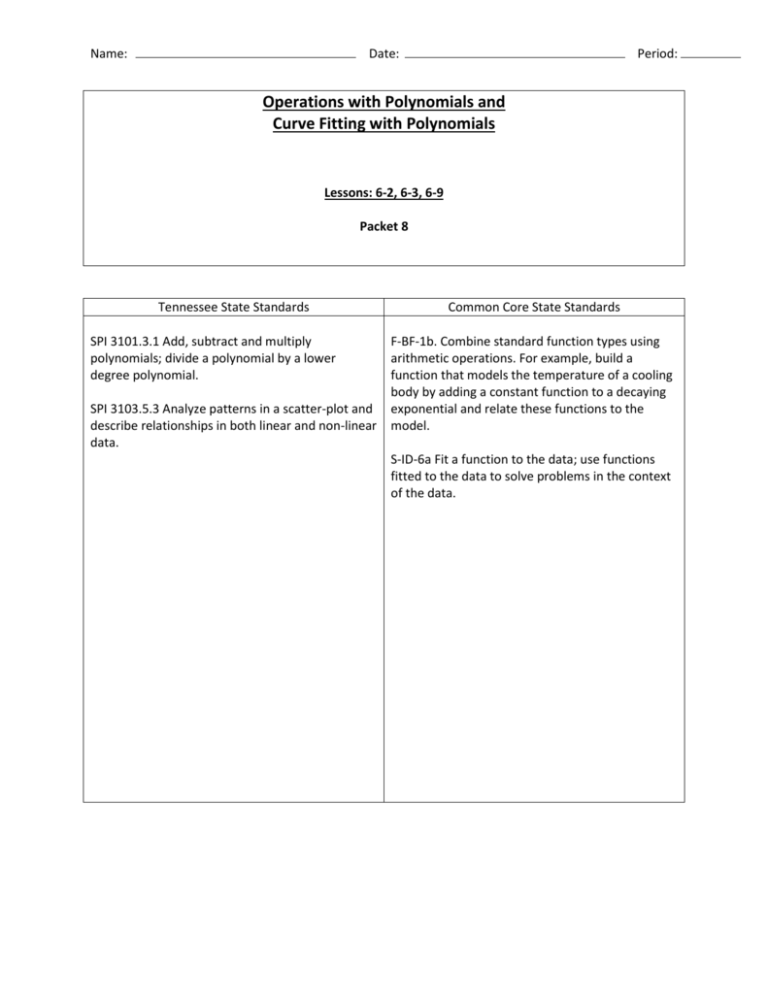
Name:
Date:
Period:
Operations with Polynomials and
Curve Fitting with Polynomials
Lessons: 6-2, 6-3, 6-9
Packet 8
Tennessee State Standards
SPI 3101.3.1 Add, subtract and multiply
polynomials; divide a polynomial by a lower
degree polynomial.
SPI 3103.5.3 Analyze patterns in a scatter-plot and
describe relationships in both linear and non-linear
data.
Common Core State Standards
F-BF-1b. Combine standard function types using
arithmetic operations. For example, build a
function that models the temperature of a cooling
body by adding a constant function to a decaying
exponential and relate these functions to the
model.
S-ID-6a Fit a function to the data; use functions
fitted to the data to solve problems in the context
of the data.
Name:
Date:
Lesson 6-2
Multiplying Polynomials
Period:
p.1
Warm-Up: Multiply Coefficients and Add Exponents of Like Bases.
x(x3)
2(5x3)
xy(7x2)
3x2(-x5)
Monomial times a Polynomial
4y2(y2 + 3)
fg(f4 + 2f3g – 3f2g2 + fg3)
Binomial times a Binomial (FOIL)
(x + 3) (x – 5)
(x – 4) (x + 4)
Polynomial times a Polynomial
(x – 3)(2 – 5x + x2)
(y2 – 7y + 5)(y2 – y – 3)
Name:
Lesson 6-2
Date:
Multiplying Polynomials
Period:
p.2
Binomial Expansion
( x + y)2
(a + 2b)3
Part B: Homework
1. 7x(2x + 3)
2. (x + 1)4
3. (x – 1)(2x2 + 3)
4. (x – 6)(x4 – 2x3 + 1)
5. 2xy(3y2 – xy + 7)
6. (x4 + x2y)(x3 + y2)
Name:
Lesson 6-3
Date:
Synthetic Division
Dividing Polynomials with Synthetic Division
(2x2 + 7x + 9) ÷ (x + 2)
(x2 + 5x + 6) ÷ (x + 1)
(x4 – 7x3 + 9x2 – 22x + 25) ÷ ( x – 6)
Period:
p.3
Name:
Lesson 6-3
Date:
Synthetic Division
Period:
p.4
Part A: Guided Practice
(x4 – 2x3 + 3x + 1) ÷ (x – 3)
(3x2 + 9x – 2) ÷ (3x – 1)
Name:
Lesson 6-3
Date:
Dividing Polynomials
Period:
p.5
Part B: Homework (Use Synthetic Division)
1. (x2 – 18x + 14) ÷ (x – 1)
2. (3x3 – 11x2 – 56x – 48) ÷ (3x + 4)
3. (x3 – 2x – 8) ÷ (x – 2)
4. (3x3 + 5x2 + 2x – 12) ÷ (x + 3)
Name:
Date:
Adding/Subtracting Polynomials
Period:
p. 6
When adding polynomials, simply ______________ __________ _____________.
1. (x3 – 2x2 + 4x – 2) + (x2 + 3x + 5)
2. (3x4 + x2 – 5x + 8) + (-5x4 + 3x3 + 7x2 – 2x – 1)
When subtracting polynomials, _________________ the subtraction sign and
then __________________ _____________ _____________.
1. (3x4 + 5x2 – 4x + 1) – (2x4 – x3 + 2x2 + 3x – 2)
2. (-2x3 + 8x2 + x – 3) – (5x3 + 6x2 – 4x + 3)
Name:
Date:
Adding/Subtracting Polynomials
Part B: Homework
1. (2x2 + 6x + 5) + (3x2 - 2x – 1)
2. (x4 + 2x3 – 4x + 6) + (-3x4 + 4x3 +1)
3. (4x3 + 2x2 – 4x + 1) – (x3 – 4x2 + 5x + 5)
4. (4x3 – 4x2 + 3x – 1) + (2x2 + x – 3)
5. (-3x2 + 2x – 4) – (6x2 – 3x – 3)
Period:
p. 7
Name:
Date:
Lesson 6-9
Period:
Curve Fitting
p. 8
To create a mathematical model for data, you will need to figure out what type of
function is ______________________________. Finite ________________ can be
used to identify the __________________ of any polynomial data.
This chart will help you decide which type of function to use:
Function Type
Linear
Quadratic
Cubic
Quartic
Quintic
Constant Finite Differences
Degree
Example:
x
y
2
-2
5
0
8
2
11
4
14
6
17
8
1. Find the differences in the y-values.
x
y
-6
-30
-4
15
-2
30
0
34
2
41
4
60
Name:
Date:
Lesson 6-9
Period:
Curve Fitting
p.9
2. Find the differences in the y-values.
X
y
-2
-10
-1
-4
0
-1.4
3. Find the differences in the y-values.
x
4
6
8
Y
-2
-4.3
8.3
1
0
10
10.5
2
2.4
12
11.4
3
8
14
11.5
Once you know which type of function to use, use the calculator to write a
function.
1. Enter data on L1 and L2 (Stat Edit)
2. Go to Stat,Calc, and choose the appropriate type.
3. Enter- now put the function’s equation together.
1. The table shows the population of a city from 1960 to 2000. Write a
polynomial function for the data.
Year
1960
1970
1980
1990
2000
Population 4,267
5,185
6,166
7,830
10,812
(thousands)
Name:
Date:
Lesson 6-9
Curve Fitting
Period:
p.10
2. The table below shows the opening value of a stock on the first day of
trading in various years. Use a polynomial model to estimate the value of
the first day of trading in 2000.
Year
1994
1995
1996
1997
1998
1999
Price ($) 683
652
948
1306
863
901
Type of Model: ____________________________________
Equation: _________________________________________
Estimate the value of the first day of trading in 2000: ______
3. The table below shows the number of infected patients at various stages of
a flu outbreak. Use a polynomial model to estimate the number of infected
patients after 120 hours.
Time (h) 12
24
48
96
144
240
Patients 21
301
679
973
562
320
Type of Model: _______________________________
Equation: ____________________________________
Estimate the number of infected patients after 120 hours: _________
Name:
Date:
Lesson 6-9
Curve Fitting
Period:
p.11
Part B: Homework
1. Use finite differences to determine the
degree of the polynomial that best
describes the data.
x 8
10 12
14
16
18
y 7.2 1.2 -8.3 -19.1 -29 -35.8
2. Write a polynomial function
using the given data.
x
y
5
30
10
34
15
36
20
36
25
34
Type of model:
Equation:
3. The table shows the population of a
bacteria colony over time. Write a
polynomial function for the data and
use it to estimate the number of
bacteria after 7 hours.
Time (h) 1 2
3
4
5
Bacteria 44 112 252 515 949
Type of model:
Equation:
Estimate the number of bacteria after 7
hours.
4. Use finite differences to
determine the degree of the
polynomial that best describes
the data.
x
y
-2 -3
-1 1
0
4.3
1
6.9
2
8.8
3
10