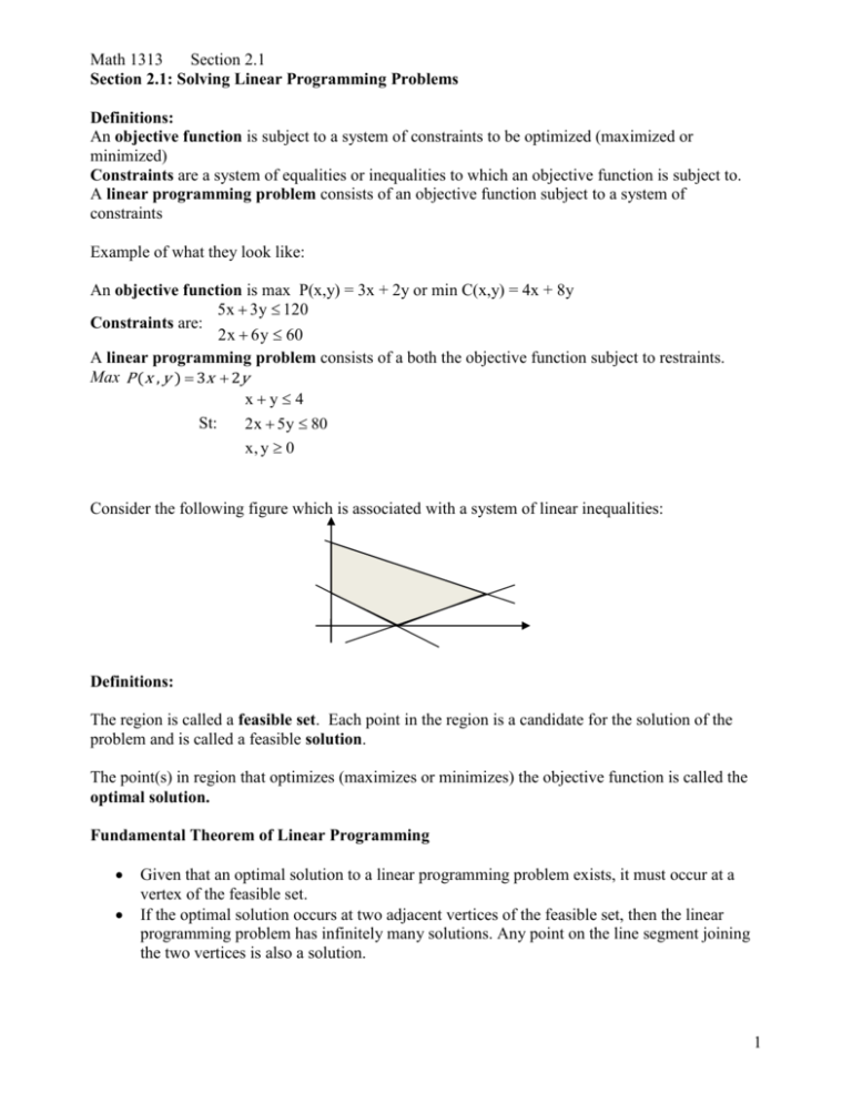
Math 1313
Section 2.1
Section 2.1: Solving Linear Programming Problems
Definitions:
An objective function is subject to a system of constraints to be optimized (maximized or
minimized)
Constraints are a system of equalities or inequalities to which an objective function is subject to.
A linear programming problem consists of an objective function subject to a system of
constraints
Example of what they look like:
An objective function is max P(x,y) = 3x + 2y or min C(x,y) = 4x + 8y
5x  3y  120
Constraints are:
2 x  6 y  60
A linear programming problem consists of a both the objective function subject to restraints.
Max P ( x , y )  3x  2 y
xy4
St:
2 x  5 y  80
x, y  0
Consider the following figure which is associated with a system of linear inequalities:
Definitions:
The region is called a feasible set. Each point in the region is a candidate for the solution of the
problem and is called a feasible solution.
The point(s) in region that optimizes (maximizes or minimizes) the objective function is called the
optimal solution.
Fundamental Theorem of Linear Programming


Given that an optimal solution to a linear programming problem exists, it must occur at a
vertex of the feasible set.
If the optimal solution occurs at two adjacent vertices of the feasible set, then the linear
programming problem has infinitely many solutions. Any point on the line segment joining
the two vertices is also a solution.
1
Math 1313
Section 2.1
This theorem is referring to a solution set like the one that follows:
Maximum
Minimum
The Method of Corners
1. Graph the feasible set.
2. Find the coordinates of all corner points (vertices) of the feasible set.
3. Evaluate the objective function at each corner points.
4. Find the vertex that renders the objective function a maximum (minimum). If there is only one
such vertex, then this vertex constitutes a unique solution to the problem. If the objective function
is maximized (minimized) at two adjacent corner points of S, there are infinitely many optimal
solutions given by the points on the line segment determined by these two vertices.
Example 1: Given the following Linear Program, Determine the vertices of the feasible set.
Max profit P ( x , y )  12x  10 y
15x  10 y  1380
Subject to: 10 x  12 y  1320
x, y  0
2
Math 1313
Section 2.1
Example 2: Given the following Linear Program, Determine the vertices of the feasible set
Min D3  3x  y
10 x  2 y  84
Subject to: 8x  4 y  120
x, y  0
3
Math 1313
Section 2.1
Example 3: Given the following Linear Program, solve for the optimal solution.
Min
C (x , y )  1200x  100y
40 x  8 y  400
Subject to:
3x  y  36
x, y  0
4
Math 1313
Section 2.1
Example 4: Maximize the following Linear Programming Problem.
Maximize C = 6x + 20y
s.t. x + y  16
x + 3 y  36
x0
y0
5
Math 1313
Section 2.1
Example 5: Maximize the following Linear Programming Problem.
Maximize C = 2x + 6y
s. t.
x + 3y < 15
4x + y <16
x≥0
y≥0
6