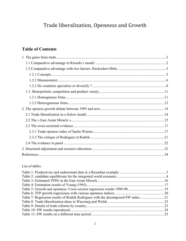
Trade liberalization, Openness and Growth
Table of Contents
1. The gains from trade ........................................................................................................................ 2
1.1 Comparative advantage in Ricardo’s model .............................................................................. 2
1.2 Comparative advantage with two factors: Heckscher-Ohlin ..................................................... 5
1.2.1 Concepts .............................................................................................................................. 5
1.2.2 Measurement ....................................................................................................................... 6
1.2.3 Do countries specialize or diversify ? ................................................................................. 8
1.3. Monopolistic competition and product variety ....................................................................... 11
1.3.1 Homogenous firms ............................................................................................................ 11
1.3.2 Heterogeneous firms ......................................................................................................... 13
2. The openess-growth debate between 1995 and now...................................................................... 14
2.1 Trade liberalization in a Solow model ..................................................................................... 14
2.2 The « East Asian Miracle »...................................................................................................... 15
2.3 The cross-sectional evidence ................................................................................................... 17
2.3.1 Trade openess index of Sachs-Warner .............................................................................. 17
2.3.2 The critique of Rodriguez et Rodrik ................................................................................. 21
2.4 The evidence in panel .............................................................................................................. 22
3. Structural adjustment and resource allocation ............................................................................... 32
References .......................................................................................................................................... 34
List of tables
Table 1: Productivity and endowment data in a Ricardian example ................................................... 3
Table 2: candidate equilibrium for the integrated world economy ...................................................... 4
Table 3: Estimated TFPG in the East Asian Miracle ......................................................................... 16
Table 4: Estimation results of Young (1993) ..................................................................................... 17
Table 5: Growth and openness: Cross-section regression results 1980-90........................................ 19
Table 6: TFP growth regressions with various openness indices ...................................................... 20
Table 7: Regression results of Rodrik Rodriguez with the decomposed SW index .......................... 21
Table 8: Trade liberalization dates in Wacziarg and Welsh .............................................................. 23
Table 9: Details of trade reforms by country ..................................................................................... 23
Table 10: SW results reproduced ....................................................................................................... 24
Table 11: SW results on a different time period ................................................................................ 25
1
Table 12: Growth and openness in panel ........................................................................................... 26
Table 13: Growth regressed in the liberalization indicator ................................................................ 30
Table 14: Growth regressed on tariff changes ................................................................................... 30
Table 15: Approach 1 with instrumental variable.............................................................................. 31
List of figures
Figure 1: Production Possibility Frontier and autarky equilibrium : Portugal..................................... 3
Figure 2: Production Possibility Frontier and autarky equilibrium : Great Britain ............................. 3
Figure 3: The gains from trade............................................................................................................. 4
Figure 4: The gains from specialisation ............................................................................................... 4
Figure 5_ Factor Endowment and PPF: The Rybczynski Theorem .................................................... 5
Figure 6: Factor Endowment and Comparative Advantage: The Heckscher-Ohlin Theorem............. 5
Figure 7: Factor endowments and revealed factor intensities .............................................................. 7
Figure 8: Comparative advantage and the survival of exports ............................................................ 7
Figure 9: Fuel exports and GDP volatility ........................................................................................... 8
Figure 10: Export concentration and the level of income .................................................................... 9
Figure 11: Concentration: Individual country trajectories ................................................................... 9
Figure 12: The export re-concentration at high levels of income ........................................................ 9
Figure 13: What are the closing export lines? ................................................................................... 10
Figure 14: Effect of an increase in the custom duty rate on capital equipment in the Solow model. 14
Figure 15: Average growthe for closed and open economies ............................................................ 17
Figure 16: convergence among closed economies............................................................................. 18
Figure 17: Convergence among open economies .............................................................................. 18
Figure 18: Growth and import tariffs ................................................................................................. 22
Figure 19: Growth and NTB coverage ratios ..................................................................................... 22
Figure 20: Time profile of growth around liberalization year ........................................................... 27
Figure 21: Time profile of investment around the liberalization year ............................................... 28
Figure 22: Decomposition of productivity growth : within-sector vs. Structural adjustment ........... 32
Figure 23: Correlation between productivity and variation in employment per sector ..................... 33
1. The gains from trade
The tradional theory of international trade suggests that:
o Trade among countries generates efficiency gains for all countries, whatever their level of
productivity.
o Countries specialize according to their comparative advantage, generating efficiencies.
1.1 Comparative advantage in Ricardo’s model
In the Ricardian model (not to be confused with the Ricardo-Viner model as we will see later, and
which has nothing to do!), The assumptions are
•
Two countries (Portugal et GB)
2
•
•
•
•
•
•
•
Two sectors (wine and drape)
Only one factor of production (labor), perfectly mobile between the two sectors
Constant returns to scale
No transport costs
No government intervention
Perfect competition (price = cost)
At the same price, consumers share their budget equally between wine and drape
Thus, in the Ricardian model comparative advantage is determined by the relative productivity of
labor, which is the only factor of production.
Table 1: Productivity and endowment data in a Ricardian example
Productivity
Portugal
UK
Wine
8
1
Drape
4
2
Endowments
(labor)
5
20
Figure 1: Production Possibility Frontier and autarky equilibrium : Portugal
Wine
40
Indifference Curve
Point of Consumption in Autarky
PPF (Production Possibility Frontier)
Drape
20
Figure 2: Production Possibility Frontier and autarky equilibrium : Great Britain
3
Wine
PPF
Point of Consumption in Autarky
20
Indifference Curve
Drape
40
Equilibrium in the world market after openess of the two economies
Table 2: candidate equilibrium for the integrated world economy
Production
Portugal
UK
Total
Wine
40
0
40
Drape
0
40
40
Consumption
Wine
20
20
40
Drape
20
20
40
Figure 3: The gains from trade
Wine
Indifference Curves
PPF
World Price Line
export
import
Drape
Figure 4: The gains from specialisation
4
Wine
Point of Production
Indifference Curves
Lines of World
prices
PPF
Drape
1.2 Comparative advantage with two factors: Heckscher-Ohlin
1.2.1 Concepts
Figure 5_ Factor Endowment and PPF: The Rybczynski Theorem
Steel
The impact of foreign investments
PPF initial
The impact of immigration
Textile
Figure 6: Factor Endowment and Comparative Advantage: The Heckscher-Ohlin Theorem
5
Point of production after structural adjustment
Indifference curves
Steel
“trade
triangle”
Relative Price on world market
(tissu moins cher)
Point of consumption after structural adjustment
PPF
Autarky relative price
Textile
1.2.2 Measurement
When there are more goods than factors of production, in general the direction of trade (who
exports what) is not determined.1 However, overall countries tend to export goods corresponding
more or less to their factor endowments
Traditionally, we calculate the Balassa index of revealed comparative advantage : denote xin the
exports of product n by country i, xi the total exports of country i, xn world exports of product n,
and x world exports. The Balassa index then is:
in 
xin / xi
xn / x
The problem with this index is that it assumes that if country i exports product n, it has a
comparative advantage in this product; but the index does not use the factor endowment of country
i. Using data on factor endowments from UNCTAD, we can determine the « revealed » factor
intensity of each product by taking the average endowments of the countries that are exporting it. If
 i is the endowment of capital of country i, the capital intensity of the good n is:
 n  i in i
where in is a modified version of the Balassa index since

i
in
 1 . 2 The advantage of this
normalization is that it allows us to put together national factor endowments and the products’
revealed intensities in the same formula. If the theory is true, the exports of countries should be
relatively less scattered around their endowments.
1
Can be found in trade flows with a continuum of goods as in Dornbusch Fisher Samuelson.
Caution: If some countries subsidize the exports of products that do not correspond to their comparative advantage,
the computation is distorted (e.g. agricultural products to Europe). We must therefore correct for this bias in the
computations.
2
6
Figure 7: Factor endowments and revealed factor intensities
Pakistan 2003-5
4
10
8
6
4
6
8
10
Revealed Human Capital Intensity Index
12
12
Costa Rica 1993
2
0
0
2
Endowment point
0
50000
100000
150000
Revealed Physical Capital Intensity Index
0
200000
50000
100000
150000
Revealed Physical Capital Intensity Index
200000
Figure 7 (ctd)
Tunisie : new export products
0
50000
100000
150000
Revealed Physical Capital Intensity Index
10
8
6
4
2
0
0
2
4
6
8
10
Revealed Human Capital Intensity Index
12
12
Tunisie 2003-5
200000
0
50000
100000
150000
Revealed Physical Capital Intensity Index
200000
Moreover, the more the exported goods are far away from the factoral endowment of the countries,
the less they survive on the world markets, despite the effect is quantitatively small :
Figure 8: Comparative advantage and the survival of exports
7
2
3
4
5
6
7
Length of trade relationship and distance to CA
2
2.2
2.4
2.6
(mean) std_dist_1
(mean) length
2.8
3
Fitted values
1.2.3 Do countries specialize or diversify ?
On the other hand, the theory suggests that countries should specialize in their comparative
advantage rather that to diversify. But specialization in raw materials, for example, can be
synonymous of "imported volatility":
.8
.6
.4
.2
GAB
0
Coefficient of variation of GDP, 2000-2007
1
Figure 9: Fuel exports and GDP volatility
0
20
40
60
Fuel share in exports
80
100
Recent studies also suggest that the decline in the volatility of GDP observed in recent decades in
the United States is largely linked to the diversification of the economy (in services).
On the other hand, generally the concentration of exports follows a non-monotone path as countries
develop : first diversification, then reconcentration. We measure the concentration of exports in
similar way as we measure the concentration in income, by three indices: (i) Gini, (ii) Herfindahl,
and (iii) Theil. Here we considered the index of Theil, whose formula is :
8
1
xi  xi 
ln  

i
n
x x
T
(1)
8
Figure 10: Export concentration and the level of income
Uganda
2000
Predicted
6
More concentrated than
predicted
4
Uganda
2010
2
Less
concentrated
than predicted
0
20000
40000
60000
GDP per cap, 2005 PPP dollars
Theil index
Fitted values
80000
Theil index, Uganda
And the reconcentration ocurred in the individual trajectories of countries :
4
5
Figure 11: Concentration: Individual country trajectories
IRL
3
GRC
2
ESP
15000
GBR
20000
25000
30000
35000
GDP per capita, PPP (constant 2005 international $)
40000
Which countries are those that re-concentrate?
Figure 12: The export re-concentration at high levels of income
9
7
5000
6
4000
5
Theil index
3000
2000
4
Theil index
3
0
1000
number of exported products
# active export lines
0
20000
40000
GDP per capita PPP (constant 2005 international $)
60000
Active lines - quadratic
Active lines - non parametric
Theil index - non parametric
Theil index - quadratic
How can we explain the reconcentration? Essentially the inertia of trade flows, export lines that are
closed have factor intensities corresponding to weaker endowments than those of countries that
close. For example, the average of trade lines closed by the EU corresponds to the combined
endowment of human and physical capital of Indonesia. These lines should be long gone, but they
remain open by inertia.
Figure 13: What are the closing export lines?
2
4
6
8
10
12
Human capital
0
50000
100000
Product intensities
150000
200000
Country endowments
Capital
In short, the theory seems to stick quite well with empirical observation, although the "content
factors" does appear to explain only a small part of international trade. We therefore need other
models to have a more complete view of its determinants.
On the other hand, so far everything discussed was essentially static: allocative efficiency
considerations tell us nothing about the growth. In the models of endogenous growth, growth is
mainly due to innovation ; international trade plays only an indirect role (i.e. through innovation).
10
So we will discuss the relationship between trade and growth from an essentially empirical point of
view, except a small detour to the Solow model in Section 3
1.3. Monopolistic competition and product variety
1.3.1 Homogenous firms
The monopolistic competition model
The Heckscher-Ohlin model explains trade by differences in factor endowments. It cannot explain
the trade between countries with similar endowments, and even less intra-industrial trade. We will
now focus on an alternative model proposed by Krugman (1980), called « monopolistic
competition».
The ingredients for a model of monopolistic competition are :
o Product differentiation that generates a finite elasticity for each firm
o Economies of scale
The gains of trade in the MC model come from competition, which compresses margins and prices.
Consider the following example from Krugman, Obstfeld and Mélitz (2012), pp 168-177
Let S be the volume of national trade, which we take as exogenously given (independant of the
prices of the firms active in this market) which is of course unrealistic but simplifies the analysis
greatly. Let n be the number of firms active in the market, b a parameter of demand (linear), Qi the
quantity sold per company i, pi its price and p the average price in the market.
Total cost is the sum of a fixed cost F and a marginal cost c :
Ci  F  cQi
which gives average cost of :
ACi 
F
c
Qi
(2)
Demand function facing firm i :
1

Qi  S   b  pi  p  
n

(3)
In a «symmetric equilibrium» where all firms set the same price pi  p , it can be seen from (12)
that Qi  S / n ; market shares are equal.
Optimal pricing by profit-maximizing firms equalizes marginal cost and marginal revenue. To
derive marginal revenue, invert (3) to get the demand price:
pi 
1 Qi

p
bn bS
Revenue is price multiplied by quantity
11
(4)
piQi 
Qi Qi 2

 pQi
bn bS
(5)
and marginal revenue is the derivative of revenue w.r.t. quantity:
1 2Qi

p
bn bS
1 Qi
Q


 p i
bn bS
bS
RM i 
(6)
pi
 pi 
Qi
bS
Marginal cost is simply c. Optimal pricing is therefore
pi 
Qi
c
bS
(7)
Qi
bS
(8)
Or
pi  c 
"mark-up"
In the symmetric equilibrium where all firms adopt the same price, Q = S/n , optimal pricing
simplifies to
pi  p  c 
1
bn
i
(9)
In this equilibrium, average cost is found by substituting Q = S/n in (4), which yields
AC  c 
Fn
S
(10)
With free entry, profits must be zero, which means that price has to equal average cost:
c
1
Fn
c
bn
S
(11)
S
bF
(12)
or
n2 
which determines the number of firms compatible with zero profits in the market (no incentive for
additional entry). In this model, gains from trade arise because of
o Economic integration that creates a bigger market
o Increasing competition, reducing margins
This can be seen by « merging » two countries with equal size S as part of a big-bang tradeliberalization experiment.
12
Effects of trade liberalization
We do the comparison that is commonly done in international trade between an equilibrium in
autarky and an equilibrium with free trade where all barriers are eliminated. The effect is illustrated
in a numerical example in the excel file Exemple concurrence monopolistique.xlsx. Suppose that
the two countries are of equal size and that there is no transportation cost. Then their combined size
is S '  2S , so the total number of firms is
n' 
S'
2S
S

 2
 1.414n
bF
bF
bF
and the equilibrium price and quantity are
p'  c 
Q' 
1
p
bn '
S ' 2S
S

 2  2Q  Q
n'
n
2n
So :
o The total number of varieties available to any consumer in the two-country area increases (there
are fewer in each country but consumers have access to both)
o The equilibrium price is lower, and so are profit margins (not shown but easy to calculate)
o Output per firm increases.
Damn it, everything is fine in this world?
1.3.2 Heterogeneous firms
Note that the trade liberalization induces firm exit, since n '  2n  2n . In a symmetric
equilibrium, which firms will exit is indeterminate. But suppose now that potential entrants differ in
their marginal cost ci, in accordance with new “heterogeneous-firm” models. Those with marginal
cost higher than the « choke price » don’t enter.
Intercept of demand facing each firm: Using (13), Qi = 0 implies
p choke 
1
p
bn
And the slope of the demand curve is :
dpi
1

dQi
bS
Trade liberalization means that pchoke goes down as n goes up, while the slope becomes “less
negative” as S goes up. Thus, under the effect of an increase in S and the induced increase of n, the
demand curve rotates anticlockwise.
o The demand increases for big firms with low marginal cost
o But it decreases for firms with higher marginal cost, which leads to the exit of some firms.
13
2. The openess-growth debate between 1995 and now
2.1 Trade liberalization in a Solow model
Everything that we saw at the beginning of this chapter was static. Is there any reason to think that
trade liberalisation could accelerate the growth? Yes if trade liberalization affects the price of
capital goods, for example. To see this, we take the Solow model and assume that the domestic
price of capital goods (the capital) is :
pK  pK* 1  tK 
where pk* is the world price of one unit of capital (one « machine ») and tk is the customs duty on
imported capital. Assume, to simplify, that pk*  1 , that is if we measure the capital in dollars, then
one unit is worth a dollar . Rewrite the law of motion of capital as :
K 
I
I
K 
K
pK
1  tK
Then we have :
 I 

 K
dk  1  tK 
k

 kLˆ
dt
L
 1 I
K
ˆ

    kL
L
 1  tK  L
 1

 1  tK
 
 sk    n  k .

A high customs duty therefore lowers the curve in Figure 14; the steady state (the intersection of the
curves, that are respectively representing the first term on the right of the equation above, and the
second term) moves to the left (at a level of capital per worker lower) and the rate of growth during
the transition to steady state, slows.
Figure 14: Effect of an increase in the custom duty rate on capital equipment in the Solow model
14
In the particular case of capital goods, the link between trade liberalization is therefore direct (and
obvious). This explains the 'climbing' structures of tariffs, prevailing in most developing countries :
low or zero tariff on capital goods, moderate tariff rates on intermediate products used as inputs in
the industry, and the highest rates on consumer goods.
2.2 The « East Asian Miracle »
Empirically, what can we say about the relationship between trade and growth? The « East Asian
miracle » is the title of a World Bank report published in 1994 and dedicated to the spectacular
growth of the Asian tigers (compared to other continents, in particular Africa and Latin America).
This report had considerable visibility although it was highly controversial.
The approach was a “growth accounting” one based on a Cobb-Douglass production function :
Yit  Kit Lit  H it 
yit  ln Yit 
(0.13)
Log-linearizing gives an estimable growth equation
yit   kit  
it
  hit  uit
where ui is the error term. Let ei be the residual of the estimation in (14), i.e.
15
(14)
eit  yit  ˆ kit  ˆ
it
 ˆhit
(0.15)
We will give a name to this residual : TFP (Total Factor Productivity). Taking first differences (i.e.
growth rates, since everything is in logs) we define Total Factor Productivity Growth (TFPG) as
eit  eit  eit 1  TFPGit
(0.16)
This gives us a decomposition of sources of growth in two components :
o Accumulation, i.e. what is predicted by (14),
o TFPG or improved Efficiency (the residual)
This decomposition is very important. If accumulation (especially capital) is the dominant
contribution to growth, the recipe for economic policy is the "mobilization of savings" for
investment. This can be done - and has been historically - abruptly by taxing agriculture to generate
the resources needed for investment. Extreme cases: the Soviet Union under Stalin. It is also what
inspired many economic policies in Africa.
On the other hand, if the TFPG is dominant, then is something else. The problem is that as the
TFPG is a residual, by definition it is not known what it is, and we could put what we want as
interpretation.
Table 3: Estimated TFPG in the East Asian Miracle
Average TFP
1970-90 (% per year)
Taiwan
Hong-Kong
Korea
Japan
Thailand
Singapore
Malaysia
3.76
3.64
3.10
3.48
2.49
1.19
1.07
Latin Am.
Afr. sub-sah.
0.13
-0.99
There is clearly a difference in the nature of growth between the SE Asia and the remainder (AL
and ASS). The TFPG is dominant in Asia, not elsewhere. Explanation: trade openness that forces
local businesses to restructure and improve the efficiency.
Unfortunately, the same year when the preliminary draft of the « East Asian Miracle » circulated,
Alwyn Young published a paper that showed the labour factor was improperly measured
(underestimated) for SEA (South East Asia) countries in the report of the Bank, the residual
measured correctly was a bit smaller for these countries. Even more of a miracle!
16
Table 4: Estimation results of Young (1993)
Source : Young, 1993
2.3 The cross-sectional evidence
2.3.1 Trade openess index of Sachs-Warner
Idea: correlate the growth in the period 1980-90 with a measure of trade openess. Bianary measure :
either open or closed country. « Closed » if one of more of the following criteria are satisifed:
1.
2.
3.
4.
5.
Average tariff greater than 40%
Rate of coverage of non-tariff barriers (quotas etc.) greater than 40% of imports
Black market currency premium greater than 20% during the decade
Export State Monopoly
Socialist Economy
SW found a strong correlation between growth and their measurement of the opening. Already in
descriptive statistics, the difference is clear :
Figure 15: Average growthe for closed and open economies
17
Source : Sachs Warner (1995)
In addition there is convergence among the open countries but not closed countries:
Figure 16: convergence among closed economies
Source : Sachs Warner (1995)
Figure 17: Convergence among open economies
18
Source : Sachs Warner (1995)
The cross-section regression results confirm the descriptive statistics (table 5).
Table 5: Growth and openness: Cross-section regression results 1980-90
Source : Sachs Warner (1995)
Edwards (1998) attempted to show that the results of Sachs and Warner were robust and not the
effect of a particular approach. It includes all of the openess measures (Sachs and Warner and other)
and systematically explores the correlation between these measures and the TFPG.
19
OPEN
Sachs-Warner
WDR
Openess Index of the World Bank (composite)
LEAMER
Residual of an equation of openess
BLACK
Balck market premium on currrencies
TARIFF
Average import tariff
QR
Rate of coverage of quantitative trade barriers
HERITAGE Trade-distortion perception index
CTR
Revenue on import taxes in proportion of the value of imports
WOLFF
Another residual of a regression of openess
SW results are robust; several other similar exercises give the same results
Table 6: TFP growth regressions with various openness indices
Source : Edwards 1998.
20
Basically, the message is that regardless of the measure of openess that we take, the correlation with
the TFPG seems well-established. The message of the East Asian Miracle was fundamentally
correct even if the measures are differentgood this is.
2.3.2 The critique of Rodriguez et Rodrik
Rodriguez et Rodrick (2001) show the opposite. They do an exercise of brutal deconstruction of all
this econometrics, in particular of the econometrics of Sachs Warner.
1 si tariffs < 40% & NTB < 40% et pas SOC
SQT  
sinon
0
1 si BMP < 20% & pas de MON
BM  
sinon
0
Table 7: Regression results of Rodrik Rodriguez with the decomposed SW index
21
Figure 18: Growth and import tariffs
Source : Rodriguez et Rodrik (2001)
Figure 19: Growth and NTB coverage ratios
Source : Rodriguez et Rodrik (2001)
So what explains the differences of TFPG, is not so much trade policy stricto sensu, but rather
macroeconomic policy (the overvaluation of the exchange rate measured by the premium on
currencies) and export monopolies. But what country had exchange rates overvalued in the 1980s?
But that had exchange rates overvalued in the 1980s? Latin America. Which country had export
monopolies? Africa.
2.4 The evidence in panel
22
All first generation studies were cross-sectional. Wacziarg and Welsh (2008) remake the estimates
in panel data by carefully identifying the date of trade liberalization (while SW did not date, since
they were using a cross-sectional over a decade). Employing a panel allows to use the fixed-effects
estimator (dummy variables that capture country-invariant characteristics over time). The effect is
much better identified, as it is "within-country" that is to say, it filters the heterogeneity between
countries due to unrelated trade openness factors.
Table 8: Trade liberalization dates in Wacziarg and Welsh
Table 9: Details of trade reforms by country
23
Results : Reproducing exactly the exercise of SW, they find the same findings :
Table 10: SW results reproduced
24
Contrariwise, when running the same regressions on another time period (the 90s) , nothing stays
significant :
Table 11: SW results on a different time period
25
What to make of it? The answer comes with panel regressions where the fundamental explanatory
variable is the date of trade liberalization; the date of the liberalization contains additional
information that is not distorted by other unexplained differences between countries entre pays
(since we use the difference in time for each country).
Table 12: Growth and openness in panel
26
Once doing this, the results become correct for all periods – far more convincing. Figure 20
displays the results in a more intuitive way. Time is normalized to be zero in the year of trade
liberalization for each country (so if Colombia liberalises in 1995, 1994 = -1, 1995 = 0, 1996 =
1 for Columbia ; if Chile liberalises in 1970, 1969 = -1 etc.). Each point on the curve is the average
of the sample growth at t = -10, t = -9, etc. We observe an accelaration of growth of about 1.5
percentage points around the year zero.
Figure 20: Time profile of growth around liberalization year
27
Figure 21 shows the same finding for investment. We observe a spectacular rise in the rate of
investment after the liberalization.
Figure 21: Time profile of investment around the liberalization year
On the other hand, the identification problem remains still unsolved in Wacziarg and Welsh due to
the fact that the trade reforms were often implemented at the same time as reform packages that
affected several other sectors of the economy (macroeconomic stabilizations, privatizations,
governance reforms, etc.) and oftentimes also coincide with changes in government. So : is it really
the trade liberalization causing the effects or other simultaneous developments?
Estevadeordal et Taylor (2009) revisited the question in the different ways where the second one is
interesting in itself to understand for the used methodology.
Approach 1 (« simple differences »)
The regress the change in growth on the change in tariffs in a panel of countries—a standard
technique. With i representing a country, t the time, git the growth of country i at time t,
28
xit  hit , zit  a country-specific vector (human capital and characteristics of governance), and  it the
average of tariffs of country i in time t.
git  git  gi ,t 1
(17)
And the same for other variables put in differences. The equation becomes
git  0  1gi ,t 1  xit α2  3 ln 1   it   uit
(18)
Approach 2 (« differences in differences »)
E&T use as natural experiment the liberalization implemented by a number of countries during
trade negotioations in Uruguay (the « Uruguay Round » that took place between 1986 and 1994).
Certain countries liberalized their tariffs; they form the « treatment group » ; other countries that
didn’t liberalize are put in the « control group ». Again, the sample structure is a panel, but now the
estimation technique is called « differences in differences ». This term expresses that we compare
the performance before and after a certain date where the treatment starts (the first difference), but
for two groups, the treatment and the control group (second difference). This estimation technique
is commonly used in medical sciences.
With Di being a dummy variable marking belonging to the treatment group and Tt the treatment
period (after the Uruguay round) ; so
1 if t  1994
Tt  
0 if t < 1994
The basic equation becomes
git  0  1Di   2Tt  3  Di  Tt   xi 0α4  uit
(19)
Treatment _ effect
And the coefficient  3 gives the treatment effect. We can also re-write (19) in a simpler way with
fixed effects for countries and years:
git    Di  Tt    i   t  uit
(20)
Treatment effect
Finally a third way of writing and estimating this equation consists of defining two long periods (
t0  1975  1989 and t1  1990  2004 ), which gives us a two-period panel, and taking the change
between those two periods :
gi  gi ,t1  gi ,t0
(21)
gi   0  1 gi ,t0  x i α 2   3 Di  ui
(22)
Which yields
The basic results of the Diff-in-Diff approach (DD) are displayed in Error! Reference source not
ound.. The first column uses the average of tariffs for all goods as regressor of interest (« liberalizer
indicator »); the second column uses the average of tariffs only on consumption goods, the third
29
uses the average on tariffs on equipment goods and the fourth uses the average tariff on
intermediate goods. We find that the coefficients are significant and estimated more precisely for
the equipment goods than for consumption goods. However, the effects are rather weak.
Table 13: Growth regressed in the liberalization indicator
The results of the first approach are very similar, but with the opposite sign since lower tariffs
accelerate growth :
Table 14: Growth regressed on tariff changes
30
Again, the coefficients are very small (signalizing a very weak effect) and only significant at the
10% level (signalizing that the effect is not well measured). Contrariwise, the coefficient on the
tariffs for equipment good sis two times higher than the coefficient for consumption goods, which is
in line with the basic growth model of section 2.1.
Endogeneity
The two approaches face similar problems, firstly endogeneity and secondly selection. They only
handle the first problem, where the problem is that the variation in tariffs and the variation in
growth could be explained by the same omitted variable, for example a change in government.3
The instrumental variable is the interaction between two things:
1. The intensitiy of the Great Depression in the observed countries
2. The level of tariffs in the countries before the Uruguay round.
The idea of the first element is that suffered more in the Depression have more than others lost the
faith in liberalism and adopted more protectionist policies afterwards, which could have survived
until today and resulted in less willingness for a liberalization. The idea of the second element is
that for liberalzing, countries must have entered the Uruguay round with high tariffs (otherwise no
need for liberalization) So low intensity of the Great Depression × high level of tariffs predict a
strong liberalization in the Uruguay round.
Table 15: Approach 1 with instrumental variable
3
In the seond approach, we face a selection problem. The approach relies on the hypothesis that the decision to take the
treatment is uncorrelated with the potential effect of the treatment. In fact, if the countries that liberalized were
systematically more likely to benefit from the treatment, we cannot use the equation (7) to deduct that the same effect
would have worked in the countries that were not treated. Therefore we have to control for this selection effect that is
always present when the treatment is not given at random, but this control is not done here.
31
We note that the effect is now stronger and more significant (it’s the « second stage » that we care
about; we have -0.05 now vs. -0.03 before, and the effect is significant at 5%).
3. Structural adjustment and resource allocation
Is this the end of the debate ? Not yet. In a recent paper, McMillan et Rodrik (2010) have
decomposed the growth of productivity and shown a result opposing the message of the beginning
of the course :
o The productivity growth in a sector is comparable across countries ; particularly there is no
substantial difference between Africa and America as before
o In contrast, in favour of a structural adjustment : in these two regions ressources have moved
from sectors with high productivity growth towards sectors with low productivity growth.
Supposing that the productivity of the manufacturing sector was a weighted average of the
productivity of several sectors.
qt   j  j q j
with

j
j
 1 . We can express its variation, qt  qt  qt 1 as
q 
  q
j
j
j
Croissance "within"


j
q j  j   j  j q j
Structural adjustment
small--we ignore it!
Representing the first term in grey and the second in black in averages per region, McMillan and
Rodrik (2011) obtain in Figure 22:
Figure 22: Decomposition of productivity growth : within-sector vs. Structural adjustment
32
Source : McMillan and Rodrik (2011).
The grey component doesn’t really vary from one region to the other. However, the black part
really makes a difference. The structural adjustment has moved resources to the wrong place! The
case of Argentina is particularly interesting (Figure 23).
Figure 23: Correlation between productivity and variation in employment per sector
Source : McMillan and Rodrik (2011).
33
References
Edwards, Sebastian (1998); “Openness, Productivity and Growth: What Do We Really Know?”;
Economic Journal 108, 383-98.
Estevadeordal, Antoni, and Alan Taylor (2009), “Is the Washington Consensus Dead? Growth,
Openness, and the Great Liberalization, 1970s-2000s”; IDB working paper IDB-WP-I38;
Washington, DC: Inter-American Development Bank.
McMillan, Margaret S. and Dani Rodrik, “Globalization, Structural Change and Productivity
Growth,” Working Paper No. 17143, NBER (http://www.nber.org/papers/w17143), June 2011.
Rodrik, Dani, and F. Rodriguez (2001), “Trade Policy and Economic Growth: A Skeptic's Guide to
the Cross-National Evidence”; in Ben S. Bernanke and Kenneth Rogoff, editors, NBER
Macroeconomics Annual 2000, Volume 15, p. 261 – 338; Boston, MA: National Bureau of
Economic Research.
Sachs, Jeffrey, and Andrew Warner (1995), “Economic Reform and the Process of Global
Integration”; Brookings Papers on Economic Activity 26, 1-118.
Wacziarg, Romain, and K. Welch (2008), “Trade Liberalization and Growth: New Evidence”;
World Bank Economic Review 22, 187-231.
The World Bank (1993), The East Asian miracle : economic growth and public policy; Washington,
DC: The World Bank.
34