[ kd ]
hwk06ans
Ast 4001, Oct-Nov 2015
Answers for homework set 6 -- Stellar interiors, homology relations, H-R diagram
_______________________________________________________________________________________
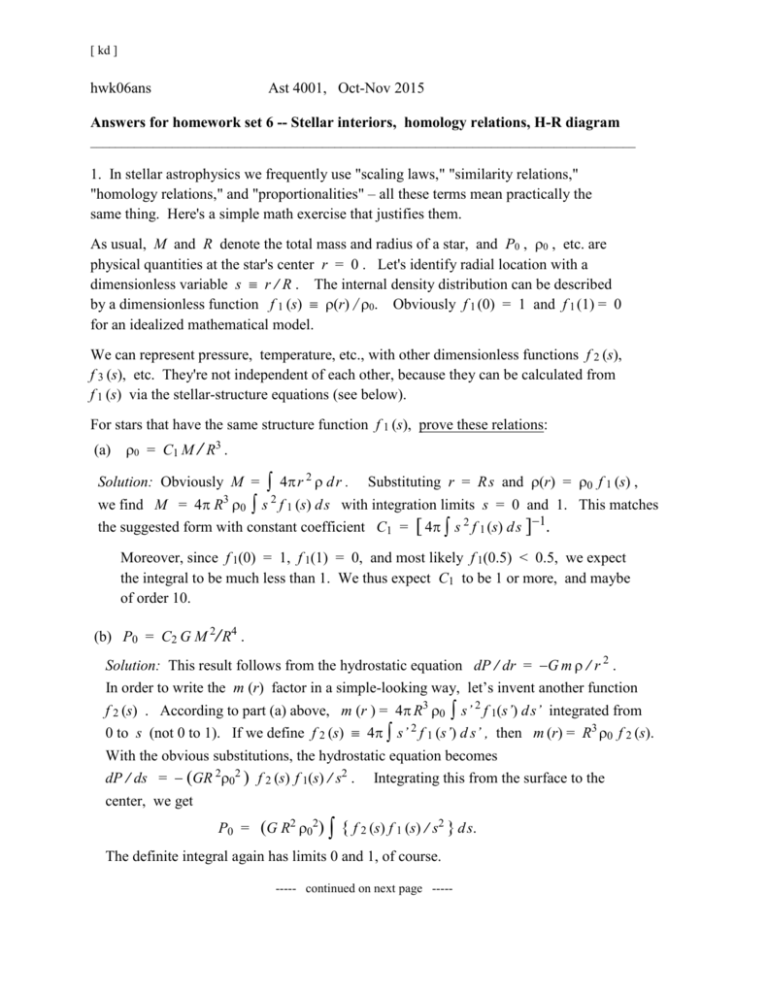
1. In stellar astrophysics we frequently use "scaling laws," "similarity relations,"
"homology relations," and "proportionalities" – all these terms mean practically the
same thing. Here's a simple math exercise that justifies them.
As usual, M and R denote the total mass and radius of a star, and P0 , 0 , etc. are
physical quantities at the star's center r = 0 . Let's identify radial location with a
dimensionless variable s  r / R . The internal density distribution can be described
by a dimensionless function f(s)  (r) / 0. Obviously f(0) = 1 and f(1) = 0
for an idealized mathematical model.
We can represent pressure, temperature, etc., with other dimensionless functions f(s),
f(s), etc. They're not independent of each other, because they can be calculated from
f(s) via the stellar-structure equations (see below).
For stars that have the same structure function f(s), prove these relations:
(a)
0 = C1 M / R3 .
Solution: Obviously M =  4r 2 d r . Substituting r = R s and (r) = 0 f(s) ,
we find M = 4R3 0  s 2 f(s) d s with integration limits s = 0 and 1. This matches
the suggested form with constant coefficient C1 =
[ 4 s 2 f (s) d s ].

Moreover, since f(0) = 1, f(1) = 0, and most likely f(0.5) < 0.5, we expect
the integral to be much less than 1. We thus expect C1 to be 1 or more, and maybe
of order 10.
(b) P0 = C2 G M 2/ R4 .
Solution: This result follows from the hydrostatic equation dP / dr = G m / r 2 .
In order to write the m (r) factor in a simple-looking way, let’s invent another function
f(s) . According to part (a) above, m (r ) = 4R3 0  s’ 2 f(s’) d s’ integrated from
0 to s (not 0 to 1). If we define f(s)  4 s’ 2 f(s’) d s’ , then m (r) = R3 0 f(s).
With the obvious substitutions, the hydrostatic equation becomes
dP / ds = (GR 202 ) f(s) f(s) / s2 . Integrating this from the surface to the
center, we get
P0 = (G R2 02)  { f(s) f(s) / s2 } d s.
The definite integral again has limits 0 and 1, of course.
----- continued on next page -----
4001hwk06ans - p2
----- 1(b) continued: -----
…Next, substitute the formula for 0 from part (a). Result:
P0 = (GM 2/ R 4) C12  ( f(s) f(s) / s2 ) d s .
This is the desired formula, with C2 = C12  ( f(s) f(s) / s2 ) d s .
Recall that part (a) gave a formula for C1 . So far we have accumulated a bunch of
definite and indefinite integrals. Since each of them is specified in terms of the original
function f(s) , a computer would not have any serious trouble calculating C1, then
f(s), then the definite integral shown above, and then C2, all based on one “known”
function f(s) . This business may seem confusing altogether, but each individual step
is pretty definite.
Remember that we can deduce the forms of the scaling laws merely by inspecting the
basic differential equations, without the f, f stuff! The point of this exercise is to
show that careful formal math gives the same answers as the simple informal approach.
(c) T0 = (C3 G / ) M / R .
Solution: For an ideal gas, P0 = 0T0 . Parts (a) and (b) gave us expressions for 0
and P0 . Combining all three expressions to eliminate 0 and P0, we find
T0 = (C2 G / C1 ) M / R. If we set C3 = C2 / C1, this is the requested result.
(d) E TOT = (C4 G) M 2 / R .
Solution: According to the virial theorem, E TOT = E G / 2 =  0.5
 0.5
 ( G m / r ) · 4 r 2 d r

 ( Gm / r ) dm
=  (2  G R 5 0 2 )  f(s) f(s) s d s.
Since 0 = C1 M / R3 , this sorts out to the above expression with
C4 = 2  C1 2
 f(s)
f(s) s d s.
Find a set of formulae that can be used to calculate C1 and C2 if we know f(s).
-- These were noted in the solutions for parts (a) and (b).
_______________________________________________________________________________________
----- problem 2 is on next page -----
=
4001hwk06ans - p3
_______________________________________________________________________________________
2. There are really at least two versions of the Hertzsprung-Russell diagram. The basic
fully-observational version is a plot of either spectral type or B  V color vs. magnitude
observed at some wavelength (often the absolute visual magnitude). In a “physical”
H-R diagram, on the other hand, the horizontal axis is converted to log Teff, and the
vertical axis is converted to either log(L / L sun) or, sometimes, absolute bolometric
magnitude Mbol. [Here "log" means decimal logarithm, log10 . Remember that
Mbol = 4.75  2.5 log (L / L sun).] Both transformations, spectral type  Teff and
MV  L, require calibrations based on theoretical atmosphere models. In this problem
we'll concentrate on the "physical" type of H-R diagram. Of course a straight line on this
log-log plot corresponds to a power-law relation between L and Teff

Find a good “physical” H-R diagram of this type, based on real data. (State where you found
it.) Look at the middle part of the main sequence, with luminosities between about 0.02 Lsun
and 500 Lsun , or +9 > Mbol > 2 .
(a) Estimate a best-fit power-law relation for that part of the main sequence,
i.e., find the exponent  in Teff L. (The main sequence is noticeably
curved, but measure its average log-log slope as well as you can.)
Answer: A typical reference book lists these rough values for selected spectral types.
Teff (K)
Mbol
Log Teff
Log (L/Lsun)
B5
15200
-2.7
4.182
+2.98
B8
11400
-1.0
4.057
+2.30
A2
9000
+1.1
3.954
+1.46
F0
7300
+2.6
3.863
+0.86
G8
5300
+5.1
3.724
-0.14
K5
4400
+6.6
3.644
-0.74
M0
3840
+7.4
3.584
-1.06
M5
3200
+9.6
3.505
-1.94
We can make a least-squares linear fit to Log L vs. Log Teff, or we can measure the
differences between the first two lines and the last two; either way we get slope
d (log L) / d (log T) = 7.2 , which implies L  Teff 7.2 or Teff  L 0.14 .
Note: This table predicts that the Sun should be about 30 % brighter than it
really is. The reason is that most lists of "main sequence stars" include various
ages and chemical compositions, all mixed together. In other words, the main
sequence is a region with appreciable width in the H-R diagram, not a narrow
mathematical curve.
----- continued on next page -----
4001hwk06ans - p4
----- Problem 2 continued -----
(b) Deduce the corresponding radius-luminosity relation, R L . This is a good thing
to do, because radius R is much more relevant than surface temperature when we're trying
to quantify a star's internal structure.
Answer: Start with L  R 2 Teff 4, based on the definition of Teff . Since we also
know that Teff  L 0.14 , it's easy to see that R L.
deduction from observations, not a theoretical prediction.
Note that this is a
(c) Adopting a simplified mass-luminosity relation, L M , estimate the average
dependence of central temperature T0 as a function of mass M.
Assuming that the Sun has T0 = 15 million K, estimate the central temperatures of
main-sequence stars with M = 0.5Msun and 5 Msun. Estimate their relative
luminosities, too.
Answer: First, if L M , then part (b) above indicates that R M . Next,
recall one of the most important homology relations: T0 M / R . Together these
imply T0 M  , but we should round this off to roughly T0 M  because the
assumptions are very inexact. The main point is that T0 depends only weakly on M .
This is again a deduction from observations, one of the facts that has to be explained
by nuclear-reaction theory.
0.5Msun : L  0.08 Lsun , T0  roughly 13 million K.
5 Msun : L  390 Lsun , T0  roughly 20 or 21 million K.
Thus a ratio of 5000 in luminosity corresponds to a ratio of only 1.6 in T0 .
Note: T0 M / R is important but it's also very rough. It depends on assuming
homologous interior structure and equal values of the gas constant  . Both of
these assumptions are somewhat elastic along the main sequence. And the reasoning
does not work for evolved giant stars, whose interior structures depend strongly on
mass and age. The size and density of the core varies through several orders of
magnitude after a star evolves away from the main sequence, and then its central
temperature becomes much higher than we'd naively guess from M / R .
_______________________________________________________________________________________