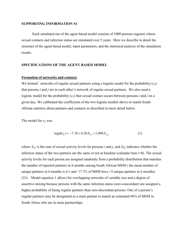
SUPPORTING INFORMATION S1
Each simulated run of the agent based model consists of 1000 persons (agents) whose
sexual contacts and infection status are simulated over 5 years. Here we describe in detail the
structure of the agent based model, input parameters, and the statistical analysis of the simulation
results.
SPECIFICATIONS OF THE AGENT BASED MODEL
Formation of networks and contacts
We formed networks of regular sexual partners using a logistic model for the probability (rij)
that persons i and j are in each other’s network of regular sexual partners. We also used a
logistic model for the probability (cij) that sexual contact occurs between persons i and j on a
given day. We calibrated the coefficients of the two logistic models above to match South
African statistics about partners and contacts as described in more detail below.
The model for rij was
logit(rij )  7.18  0.20 X ij1  1.099 X ij 2
(1)
where Xij1 is the sum of sexual activity levels for persons i and j, and Xij2 indicates whether the
infection status of the two partners are the same or not at baseline (calendar time t=0). The sexual
activity levels for each person are assigned randomly from a probability distribution that matches
the number of reported partners in 6 months among South African MSM ( the mean number of
unique partners in 6 months is 4.1 and 17.7% of MSM have >5 unique partners in 6 months)
(23). Model equation 1 allows for overlapping networks of variable size and a degree of
assortive mixing because persons with the same infection status (sero-concordant) are assigned a
higher probability of being regular partners than sero-discordant persons. One of a person’s
regular partners may be designated as a main partner to match an estimated 46% of MSM in
South Africa who are in main partnerships.
The probability that persons i and j have sexual contact on a given day, cij, was determined by
logit(cij )  10.58  10.73M ij  8.847 Rij  4.5( H i  H j )
(2)
where the indicator Mij is set to 1 if persons i and j are each other’s main partners, the indicator
Rij is set to 1 if persons i and j are regular (including main) partners, and the indicator Hi is set to
1 if person i has a main partner. The model allows for main partners to have higher contact rates
than regular partners who in turn have higher contact rates than causal (non-regular) partners.
The regression coefficients of models 1 and 2 were calibrated as follows. We searched over the
parameter space of regression coefficients by performing a grid search. For each parameter
vector in the gird, we determined how well those parameters produced patterns of sexual activity
consistent with known data from the MSM population in South Africa., Specifically, we
identified the set of coefficients (for both models 1 and 2 together) that yielded simulation
results that best matched the following available statistics on sexual networks and contacts:
mean number of unique partners in 6 months=4.1; 17.7% of persons have>5 partners; persons
without main partners had 2.7 times more partners than persons with main partners over 12
months. For each parameter vector in the grid search, we ran a simulation for 1.5 years. We
calculated simulated values of the above statistics (we used a sliding window over the 1.5 year
and performed 10 replications of the simulation . The parameters with the best match in the grid
search was determined by minimizing the sum of the squares of the percent difference between
the simulated values of the statistics and the statistics on sexual networks and contacts from data
from African studies. For example, the simulated value of the number of partners in six months
was 3.9 versus 4.1 from the observed data. The regression coefficients were chosen subject to the
constraint that the expected number of contacts per week that a person had with main and regular
partners were 3.5 and 1.0 respectively. The proportion of contacts that were UAI was adjusted to
yield an average annual HIV incidence at baseline of 6% (11-13, 23).
Inputs and Parameter Values
Attributes assigned to persons at baseline:
Each person was assigned a set of attributes at baseline (t=0).

HIV infection status (yes, no); HIV prevalence at t=0 is 25.5% (21).

On ART (yes, no); proportion on ART among HIV infected with CD4<350 at t=0 is 0.5
(21).

Knowledge of infection status (yes, no); proportion with knowledge of HIV status at t=0
is 25% (21).

Sexual role preference: persons are divided equally into three groups, either practicing
primarily insertive, receptive, or versatile sexual behaviors with probabilities of receptive
behavior on a given contact being 0.2, 0.8 and 0.5 respectively for the three groups.

HIV testing frequency: Persons are divided equally into three groups corresponding to
moderate, low, or never HIV testing frequencies with probabilities of testing within 6
months of .17, .085, and 0.0, respectively. Time between tests follow an exponential
distribution. If the CD4 of infected persons drops below 350, persons are moved into the
moderate testing group regardless of the initial group assignment.

Persons are assigned to either low or high propensity groups for engaging in UAI
(unprotected anal intercourse) on a given sexual contact with proportions 0.5 in both
groups. The probability of engaging in UAI on a given contact for the high and low
propensity groups are 1.0 and 0.4, respectively.
Daily Updates:

Annual decline in CD4 count among HIV infected is 4.26(CD4)0.5 where CD4 is current
level (26). The CD4 count at baseline ( t=0) among HIV positive persons was assumed to
follows a lognormal distribution with ln (CD4) ~ N(μ=6.2, σ=0.90). CD4 counts above
1200 are truncated. Persons were assumed to die when the CD4 count dropped below
50.

If persons learn they’re HIV positive, there’s a 1/3 decrease in their baseline frequency of
participating in UAI.

HIV transmission is simulated by Bernoulli trials using the following transmission rates:
-Transmission probability from infected insertive partner to uninfected receptive
partner is 0.014 per contact (23).
-Transmission probability from infected receptive partner to uninfected insertive
partner is 0.00175 per contact based on assuming risk of receptive behavior is
approximately 8 times that of insertive behavior. (23-25).
-The effect of PREP for uninfected persons is to reduce the probability of
transmission by 15% if person is a low adherer to PREP and 73% if person is a
high adherer to PREP. Proportions assigned to the high and low adherers groups
are each 0.5 (5, 28, 34).
-The effect of ART for HIV uninfected persons is to reduce the probability of
transmission by 96% (4).
Inputs for Network formations:

Mean number of unique partners in 6 months=4.1; 17.7% of persons have>5 partners
(21); persons without main partners had 2.7 times more partners than persons with main
partners over 12 months

Expected number of contacts per week that a person had with main and regular partners
were 3.5 and 1.0 respectively. The proportion of contacts that were UAI was adjusted to
yield an average annual HIV incidence at baseline of 6% (21).
Statistical Analysis of Simulation Results from Agent Based Model
We fit a generalized linear model to the data set of 2157 simulation results. For each of the
simulation runs we have the dependent variable y which was the proportion infected over 5 years
and the explanatory variables being the levels of the components of the intervention package. We
used a logit link function.
The modeled percentages infected over five years is given by
yˆ  100 e Z 1  e Z 
where
(3)
Z   0  1 X 1   2 X 2  3 X 3   4 X 32  5 X 33   6 X 4   7 X 2 X 4
(4)
and the X’s are the covariates that define the components of the combination HIV prevention
package. Specifically, X1 is the percentage of eligible persons who receive ART (from among
those not already receiving ART at baseline). Persons are eligible to receive ART if their
CD4<350 and had an HIV test within the preceding 6 months; X2 is the percentage of eligible
persons accepting PrEP. Persons are eligible for PrEP if they are HIV uninfected persons, had
an HIV test within the preceding 6 months and are at high risk (high risk is defined here as either
>12 acts of unprotected anal intercourse (UAI) in the preceding 6 months, or having a main
partner who is HIV infected.) X 3 is a transformation of X3 where X3 is the percentage


reductions in UAIs (specifically, X 3  100  10 100  X 3 ; see below for further explanation
and motivation for this particular transformation); X4 is set to 1 if the percentage of persons
who never received an HIV test is reduced in half from 33.3% to 16.7%.
We used iteratively reweighted least squares to account for the non-constant variance of y. The
estimated regression coefficients in equation 4 were:
Model component
coefficients (β)
Intercept
-1.0906
X1
-0.000823
X2
-0.00260
X3
-0.04184
X 32
0.000657
X 33
-0.00000879
X4
-0.0391
X2 X4
-0.000419
Each of the regression coefficients, β0,… β5, were individually statistically significant and the
main effect and interaction terms for X4 (β6 and β7) were jointly significant ( p< .01).
The final variance function that was used for the weighting was
var ( y)  0.0518 yˆ  0.1110 yˆ 3
where var(y) is the variance of the cumulative proportion infected over 5 years and ŷ is the
predicted value of y.
The confidence intervals for the percent of infections prevented given in Tables 2 and 3 were
obtained as follows. Let ε represent the proportion of infections prevented with an intervention
where the intervention is defined by a row vector of covariates X1 compared to another
intervention that is defined by a different row vector of covariates X2 As in equation 4, define
the linear predictor Z1=X1 β and Z2=X2 β where β is the vector of regression coefficients.
Then,
e Z2
e Z1

Z2
Z1
yˆ  y
  2 1  1  e Z21  e
e
y2
1  e Z2
(5)
We obtain a confidence interval for ε as follows. The first step is to obtain the variancecovariance matrix for the vector of regression coefficients β from the R programming language
which we call V (β). The second step is to calculate the 2x2 variance-covariance matrix V(Z) for
the two linear predictors Z1 and Z2. This covariance matrix is obtained using standard linear
X 
statistical theory which gives V ( Z)   1 V (β)  X 1t
 X2 
X 2t  where the superscript t represents the
transpose. The third step is to calculate the variance of ε, called var (ε), from the delta method,
which gives var( )   d  V (Z)  d t  where d, the gradient, is a row vector consisting of the first
  yˆ 1  yˆ1 
derivatives of ε with respect of Z1 and Z2. It can be shown that d   1
yˆ 2

The final step is to calculate a 95% confidence interval for ε from
  1.96 var( ) .
 yˆ1 1  yˆ 2  
.
yˆ 2

The 95% confidence interval for the percentage of infections prevented is obtained by
multiplying the endpoints of the above confidence interval by 100.
The transformation X 3 was used in the model for y (equation 4) for two reasons. First, it led to a
good fit to the observed dataset of simulation results. Second, it has a mechanistic interpretation.
The percent reduction in the probability of the occurrence of UAI on a given contact between
two partners from a prevention intervention is X3. The occurrence of a UAI requires both
partners to agree to participate in that behavior. Let X 3 = % reduction in an individual’s
probability of agreeing to participate in a UAI. Here we develop a relationship between X3 and
X 3 . Let P0i represent the probability that individual i agrees to a UAI at t=0 (that is, prior to the
prevention intervention). Suppose after the prevention intervention that probability is reduced by
X 3 % to become
 100  X 3
P1i  P0i 
 100

.

Then the probability that a given contact between persons i and j results in a UAI (assuming
independence) is:
2
 100  X 3 
 P0i P0 j 

 100  .
It follows that the percentage reduction in the probability of occurrence of a UAI (X3) expressed
in terms of X 3 is
2
 100  X 3 
X 3  100  100 
 .
 100 


Solving the above equation for X 3 we obtain X 3  100  10 100  X 3 .