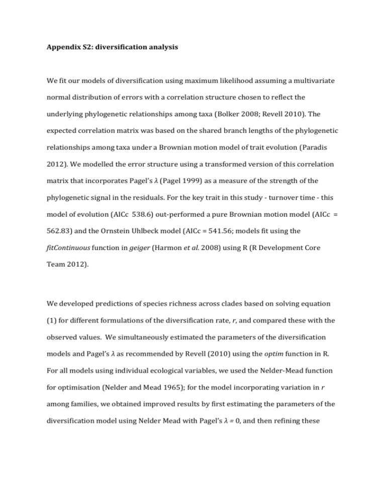
Appendix S2: diversification analysis
We fit our models of diversification using maximum likelihood assuming a multivariate
normal distribution of errors with a correlation structure chosen to reflect the
underlying phylogenetic relationships among taxa (Bolker 2008; Revell 2010). The
expected correlation matrix was based on the shared branch lengths of the phylogenetic
relationships among taxa under a Brownian motion model of trait evolution (Paradis
2012). We modelled the error structure using a transformed version of this correlation
matrix that incorporates Pagel’s λ (Pagel 1999) as a measure of the strength of the
phylogenetic signal in the residuals. For the key trait in this study - turnover time - this
model of evolution (AICc 538.6) out-performed a pure Brownian motion model (AICc =
562.83) and the Ornstein Uhlbeck model (AICc = 541.56; models fit using the
fitContinuous function in geiger (Harmon et al. 2008) using R (R Development Core
Team 2012).
We developed predictions of species richness across clades based on solving equation
(1) for different formulations of the diversification rate, r, and compared these with the
observed values. We simultaneously estimated the parameters of the diversification
models and Pagel’s λ as recommended by Revell (2010) using the optim function in R.
For all models using individual ecological variables, we used the Nelder-Mead function
for optimisation (Nelder and Mead 1965); for the model incorporating variation in r
among families, we obtained improved results by first estimating the parameters of the
diversification model using Nelder Mead with Pagel’s λ = 0, and then refining these
parameters and simultaneously estimated Pagel’s λ, using simulated annealing using the
‘SANN’ method (Belisle 1992) with 5 x 105 iterations.
#R code to perform diversification analysis based on an exponential model of
diversification where the effect of turnover times (TT) varies among families (model
15)
#estimate underlying error structure, where ‘phylogeny’ is the phylogenetic
relationships of the study taxa, of class phylo.
#uses ape package (Paradis et al. 2004)
errors<-vcv(phy=phylogeny, model="Brownian", corr=T)
#set extinction rate
ext=0
#fit model where p is a vector of model parameters and p[7] estimates Pagel’s λ.; t, is
clade age in Ma; a, whether the age relates to a stem (a=1) or crown (a=2) age; ext is the
relative extinction rate (0 or 0.9), and b(n) is a suite of dummy variables indicating
membership of n families by different clades.
#initial parameter values estimated using model excluding correlated error structure
normNLL = function(p) {
y.species = ((1-ext)*((p[1]*(1/log(TT))*b1)+
(p[2]*(1/log(TT))*b2)+(p[3]*(1/log(TT))*b3)
+(p[4]*(1/log(TT))*b4))
*(1/p[5])*(1-exp(-p[5]*t)))+log(a)
-sum(dmvnorm(log(species),mean=y.species,
sigma=p[6]*(p[7]*(errorsdiag(diag(errors)))+diag(diag(errors))),
log=T))}
out<-optim(p=c(4.9,7.7,9.8,5.9,0.04,2.04,0.5),normNLL,
control=list(maxit=500000),method="SANN")
Other models used to estimate species richness were formulated as:
Model
1
2
3
4
5
6
7
8
9
10
11
Type
Constant
Constant
Constant
Constant
Constant
Constant
Constant
Constant
Exponential
Exponential
Exponential
Description
No traits
Turnover
Dispersal
Range size
Max height
Breeding system
Turnover
Max height
No traits
Turnover
Dispersal
Family-specific?
No
No
No
No
No
No
Yes
Yes
No
No
No
12
Exponential
Range size
No
13
14
Exponential
Exponential
Max height
Breeding system
No
No
15
Exponential
Turnover
Yes
16
Exponential
Max height
Yes
Form
(p[1]*(1-ext)*t)+log(a)
(p[1]*(1-ext)*(1/log(TT))*(t))+log(a)
(1-ext)*((p[1]*Dispersal1)+(p[2]*Dispersal2)+…))*(t))+log(a)
(1-ext)*((p[1]*Range1)+(p[2]*Range2)+…))*(t))+log(a)
(p[1]*(1-ext)*(1/Ht)*(t))+log(a)
(1-ext)*((p[1]*Breeding1)+(p[2]*Breeding2))*(t))+log(a)
(1-ext)*((p[1]*(1/log(TT))*b1)+(p[2]*(1/log(TT))*b2)…)*t)+log(a)
(1-ext)*((p[1]*(1/(Ht))*b1)+(p[2]*(1/(Ht))*b2)+…*t)+log(a)
(p[1]*(1-ext)*(1/p[2])*(1-exp(-p[2]*t)))+log(a)
(p[1]*(1-ext)*(1/log(TT))*(1/p[2])*(1-exp(-p[2]*t)))+log(a)
((1-ext)*((p[1]*Dispersal1)+(p[2]*Dispersal2)+…))*(1/p[5])*(1-exp(p[5]*t)))+log(a)
((1-ext)*((p[1]*Range1)+(p[2]*Range2)+…)*(1/p[5])*(1-exp(p[5]*t)))+log(a)
(p[1]*(1-ext)*(1/(Ht))*(1/p[2])*(1-exp(-p[2]*t)))+log(a)
((1-ext)*((p[1]*Breeding2)+(p[2]*Breeding2))*(1/p[3])*(1-exp(p[3]*t)))+log(a)
((1-ext)*((p[1]*(1/log(TT))*b1)+(p[2]*(1/log(TT))*b2))+…)
*(1/p[5])*(1-exp(-p[5]*t)))+log(a)
((1-ext)*((p[1]*(1/Ht)*b1)+(p[2]*(1/Ht)*b2)+…)*(1/p[5])*(1-exp(p[5]*t)))+log(a)
In these models, Dispersal, Range and Breeding are suites of dummy variables indicating
membership of different categories of these traits for different clades (Table 1).
References
Belisle, C. J. P. (1992) Convergence theorems for a class of simulated annealing
algorithms on Rd. J. Applied Probability, 29, 885–895.
Bolker B.M. (2008). Ecological models and data in R. Princeton University Press.
Harmon L.J., Weir J.T., Brock C.D., Glor R.E. & Challenger W. (2008). GEIGER:
investigating evolutionary radiations. Bioinformatics, 24, 129-131.
Nelder, J. A. and Mead, R. (1965) A simplex algorithm for function
minimization. Computer Journal 7, 308–313.
Pagel M. (1999). Inferring the historical patterns of biological evolution. Nature, 401,
877-884.
Paradis E. (2012). Analysis of Phylogenetics and Evolution with R. Springer.
Paradis E., Claude J. & Strimmer K. (2004). APE: analyses of phylogenetics and evolution
in R language. Bioinformatics, 20, 289-290.
R Development Core Team (2012). R: A Language and Environment for Statistical
Computing. R Foundation for Statistical Computing, Vienna.
Revell L.J. (2010). Phylogenetic signal and linear regression on species data. Methods in
Ecology and Evolution, 1, 319-329.