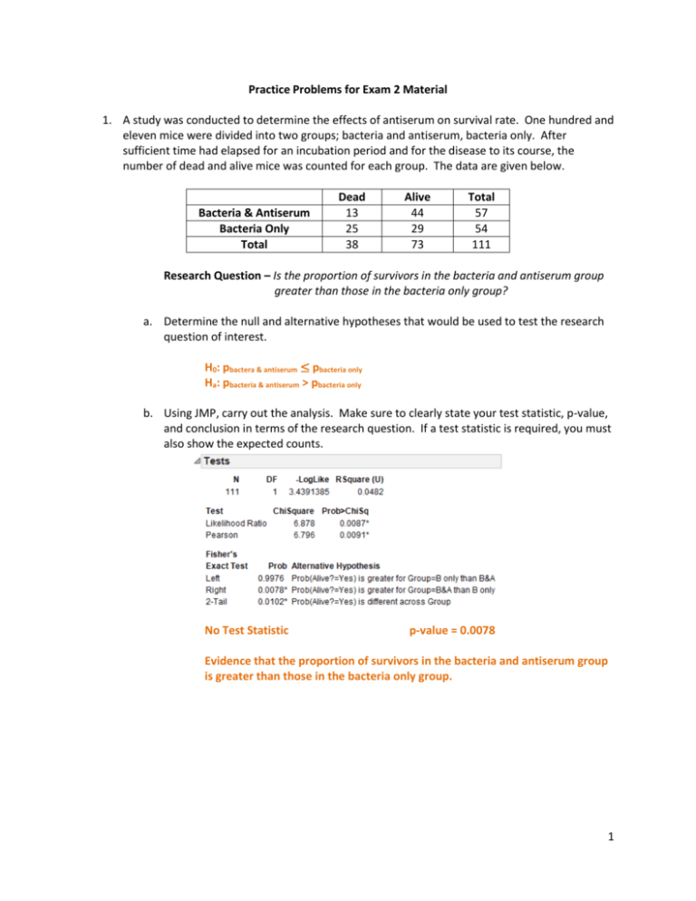
Practice Problems for Exam 2 Material
1. A study was conducted to determine the effects of antiserum on survival rate. One hundred and
eleven mice were divided into two groups; bacteria and antiserum, bacteria only. After
sufficient time had elapsed for an incubation period and for the disease to its course, the
number of dead and alive mice was counted for each group. The data are given below.
Bacteria & Antiserum
Bacteria Only
Total
Dead
13
25
38
Alive
44
29
73
Total
57
54
111
Research Question – Is the proportion of survivors in the bacteria and antiserum group
greater than those in the bacteria only group?
a. Determine the null and alternative hypotheses that would be used to test the research
question of interest.
H0: pbactera & antiserum ≤ pbacteria only
Ha: pbacteria & antiserum > pbacteria only
b. Using JMP, carry out the analysis. Make sure to clearly state your test statistic, p-value,
and conclusion in terms of the research question. If a test statistic is required, you must
also show the expected counts.
No Test Statistic
p-value = 0.0078
Evidence that the proportion of survivors in the bacteria and antiserum group
is greater than those in the bacteria only group.
1
2. During the recent economic recession, many families faced hard times financially. Some studies
observed that more people stopped buying name brand products and started buying less
expensive store brand products instead. Data produced by a recent sample of 700 adults on
whether they usually buy store brand or name brand products are given below.
Male
Female
Total
Name Brand
150
160
310
Store Brand
165
225
390
Total
315
385
700
Research Question – Is there evidence of a difference in the proportion of males and
females that buy name brand products?
a. Set up the null and alternative hypotheses that would be used to test the research
question of interest. You may write these in words or symbols.
H0: pmales = pfemales
Ha: pmales ≠ pfemales
b. Using JMP, carry out the analysis. Make sure to clearly state your test statistic, p-value,
and conclusion in terms of the research question. If a test statistic is required, you must
also show the expected counts.
Expected Counts
310
Overall % Name brand =
= 0.44
700
390
Overall % Store brand =
= 0.56
700
Male
Female
Total
Name Brand
315(0.44) =
138.60
385(0.44) =
169.40
310
Store Brand
315(0.56) =
176.4
385(0.56) =
215.6
390
Total
315
385
700
Since all expected counts ≥ 5, use Chi-square test
Test Statistic = 2.579
p-value = 0.1083
There is no statistically significant evidence (since 0.1083 > 0.05) that there is a
difference in the proportion of males and females that buy name brand
products.
2
3. University of New Mexico professor Jane hood investigated the fieldwork methods used by
qualitative sociologists (Teaching Sociology, July 2006). Searching for all published journal
articles, dissertations, and conference proceedings over the previous seven years in the
Sociological Abstracts database, she discovered fieldwork could be categorized as the following:
Interview, Observation + Participation, Observation Only, and Grounded Theory. Furthermore,
it has been hypothesized that 70% of fieldwork conducted is done by interview, 15% using
Observation + Participation, 10% using Observation Only, and 5% using Grounded Theory. The
table below summarizes the number of paper published in the last seven years that fall into
each of the above categories.
Fieldwork Method
Interview
Observation + Participation
Observation Only
Grounded Theory
Total
Number of Papers
5,079
1,042
848
537
7,506
a. Set up the null and alternative hypotheses that would be used to determine if the
observed data are consistent with the hypothesized values.
H0: pinterview = 0.70
pobservatio + participation = 0.15
pobservation = 0.10
pgroudned theory = 0.05
Ha: Two or more differ
b. Calculate the expected counts that would be used in the computation of the Chi-square
test statistic.
Interview  7506(0.70) = 5254.2
Observation + Participation  7506(0.15) = 1125.90
Observation  7506(0.10) = 750.6
Grounded Theory  7506(0.05) = 375.3
c. Using JMP, find the Chi-square test statistic and p-value for this study.
Test Statistic = 94.4023
p-value = 0.0001
d. Using the p-value from part c, is there evidence that the observed data are consistent
with the hypothesized values? Explain.
Evidence that the data do not follow the hypothesized breakdown of fieldwork
categories.
3
4. Since WSU is a laptop university which gives students the choice of either a MAC or a PC, it may
be of interest to determine whether there is a difference in the proportion of males and females
who prefer a particular brand. Therefore, a random sample of 208 female students and 122
male students was taken. Of the females selected 134 said they prefer a MAC while 66 of the
males selected said they prefer a MAC.
a. Construct a 99% confidence interval for the difference in proportions.
pˆ male =
66
= 0.54
122
Z = 2.58
(0.64 – 0.54) ± 2.58(0.06)
0.10 ± 0.15
-0.05 ≤ pfemale – pmale ≤ 0.25
134
= 0.64
208
0.54(0.46) 0.64(0.36)
= 0.06
+
122
208
pˆ female =
(0.54 – 0.64) ± 2.58(0.06)
-0.10 ± 0.15
-0.25 ≤ pmale – pfemale ≤ 0.05
OR
b. Interpret the 99% confidence interval constructed in part a.
99% confident the true proportion of females who prefer a MAC is between 0.05
smaller and 0.25 larger than the true proportion of males who prefer a MAC.
OR
99% confident the true proportion of males who prefer a MAC is between 0.25 smaller
and 0.05 larger than the true proportion of females who prefer a MAC.
c. Based on the confidence interval constructed in part a, can it be concluded that there is
a difference in the proportion of males and females who prefer a MAC laptop? Explain.
No, because 0 is included in the confidence interval.
4
5. A study was conducted to investigate gender and the most bothersome symptom for joint
disease victims. A random sample of 250 men and 300 women suspected to be joint disease
victims was taken. The data are summarized below.
Male
Female
Total
Morning Stiffness
111
102
213
Nocturnal Pain
59
73
132
Joint Swelling
80
125
205
Total
250
300
550
Research Question – Is there evidence of a relationship between gender and a person’s
most bothersome symptom for joint disease?
a. Create a mosaic plot of the data. Looking at the mosaic plot, does there appear to be a
relationship between gender and a person’s most bothersome symptom for joint
disease? Explain.
It appears there might be a relationship between gender and a person’s most
bothersome symptom because the patterns differ across gender.
b. Determine the appropriate null and alternative hypotheses that would be used to test
the research question of interest.
H0: Gender and most bothersome symptom are independent
(There is no relationship between gender and most bothersome symptom)
Ha: Gender and most bothersome symptom are not independent
(There is a relationship between gender and most bothersome symptom)
5
c. Using JMP, carry out the remainder of the test. Make sure to clearly check the
conditions, indicate the value of the test statistic, p-value, and the conclusion in context
of the research question.
Expected Counts:
213
% Stiffness =
= 0.39
550
132
% Nocturnal =
= 0.24
550
205
% Swelling =
= 0.37
550
Male
Female
Total
Morning Stiffness
250(0.39)
97.5
300(0.39)
117
213
Nocturnal Pain
250(0.24)
60
300(0.24)
72
132
Joint Swelling
250(0.37)
92.5
300(0.37)
111
205
Total
250
300
550
All ECs ≥ 5 so Chi-square test is appropriate!
Test statistic = 7.258
p-value = 0.0265
There is evidence that gender and a person’s most bothersome symptom are not
independent. That is, there IS a relationship between gender and a person’s most
bothersome symptom.
6
6. A study was done to compare the side effects of taking a new drug. Two hundred individuals
were chosen for the study and half were assigned to take the drug and the other half were
assigned to take a placebo. Of those given the drug, 10 experienced a headache, while only 5 of
those given the placebo experienced a headache.
a. Fill in the contingency table below for this scenario.
Drug
Placebo
Total
Headache
10
5
15
No Headache
90
95
185
Total
100
100
200
b. Using JMP, find the relative risk of experiencing a headache for those taking the drug
compared to those taking the placebo.
c. Interpret the relative risk found in part b.
The risk/probability of a headache for those taking the drug is 2 times more
than the risk/probability of a headache for those taking the placebo.
d. Looking at the relative risk found in part b, can you conclude there is a
relationship/difference/association in the risk of experiencing a headache for those
taking the drug compared to those taking the placebo? Explain.
Yes, because the RR ≠ 1
e. Using JMP, find the odds ratio for this scenario.
f.
Interpret the odds ratio found in part e.
The odds of NO headache for those taking the drug is 0.47 times greater than
the odds of NO headache for those taking the placebo.
7