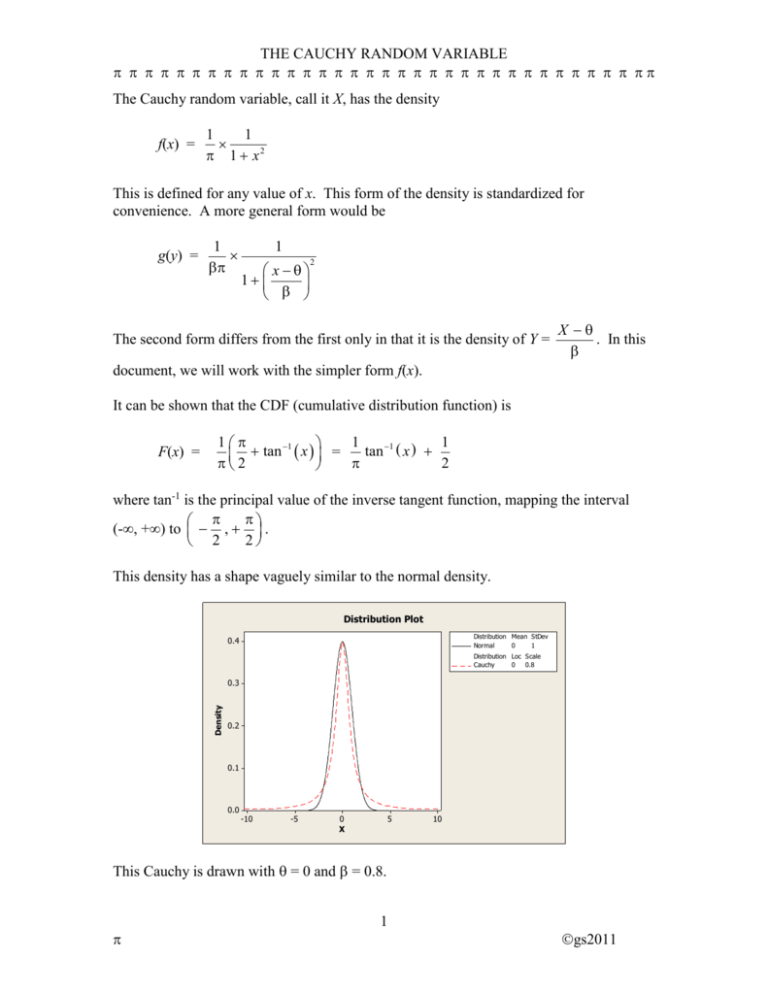
THE CAUCHY RANDOM VARIABLE
                                 
The Cauchy random variable, call it X, has the density
f(x) =
1
1

 1  x2
This is defined for any value of x. This form of the density is standardized for
convenience. A more general form would be
g(y) =
1


1
 x 
1 

  
2
The second form differs from the first only in that it is the density of Y =
X 
. In this

document, we will work with the simpler form f(x).
It can be shown that the CDF (cumulative distribution function) is
F(x) =
1
1
1

1
tan 1  x  
  tan  x   =

2
2

where tan-1 is the principal value of the inverse tangent function, mapping the interval

 
(-∞, +∞) to   ,   .
2
 2
This density has a shape vaguely similar to the normal density.
Distribution Plot
Distribution Mean StDev
Normal
0
1
0.4
Distribution Loc Scale
Cauchy
0
0.8
Density
0.3
0.2
0.1
0.0
-10
-5
0
X
5
10
This Cauchy is drawn with  = 0 and  = 0.8.

1
gs2011
THE CAUCHY RANDOM VARIABLE
                                 
The first important observation about this random variable is that its expectation
(meaning expected value, E X , does not exist. If we tried to compute the expectation, we
would go through the following steps:

EX =



0
x
1
1
1
x
1
x

dx =
dx 
dx
2
2


 1 x
  1  x
 0 1  x2
 u  1  x2 
= 

 du  2 x dx 
 1

 
1


du
u

1



1
du 
1
= 
u 



1
du
u

1



1
du
u
In this final form, the first integral is -∞ and the second integral is +∞. A difference of
the form -∞ + ∞ is undefined. Thus, we conclude that the expected value of the Cauchy
random variable does not exist.
A few notes about this derivation:
*
We might have claimed to be doing an integral in which the integrand is odd,
meaning w(-t) = -w(t). Such an integral, it might seem, must have the value 0.
However, in order to claim the value of zero, we must have the condition
M

w  t  dt   for every value M, including M = ∞. This fails for our
M
case at M = ∞. (The proper method of evaluation requires breaking the integral
into positive and negative pieces, as was done above.)
*
“E(X) does not exist” should be distinguished from the condition “E(X) = ∞.”
1
I  x  1 will have
The random variable W with density h(w) =
1  x2
E(W) = ∞. Simulations of the random variable W will have running averages that
tend to infinity. Running averages of a Cauchy random variable, as illustrated
later, will drift aimlessly.
*
Once we have shown that E(X) does not exist or E(X) = -∞ or E(X) = ∞, then we
know that there are no finite higher moments. Specifically, we cannot have E(X r)
finite for any positive integer r.
*
Since X does not possess finite moments, it does not have a moment generating
function.

2
gs2011
THE CAUCHY RANDOM VARIABLE
                                 
A fascinating property of the Cauchy distribution is that the average of a sample of n has
the same probability law as a single observation. That is, the density f(x) given at the
start of this document is also the density of the average of a sample of n. This fact can
be proved easily using characteristic functions (the complex version of moment
generating functions) but will not be shown here.
As a consequence, sample averages do not collapse to a single number, and do not
furnish consistent estimates. You might find it reassuring to learn that the sample median
still converges to the population median.
It is insightful to examine simulations of Cauchy random variables. The following is a
list of 100 random observations from the density f(x) :
-1.5139
0.4686
0.3985
-3.5293
-2.1019
0.1694
1.2675
-2.7102
0.9599
10.2059
-2.4118
0.3133
-6.4196
-11.4843
-0.8738
-0.1901
3.9489
-0.1446
-2.6524
1.2915
-0.0614
-1.4026
2.3671
1.4377
1.4793
-0.6400
-0.2560
0.6219
3.4551
-2.1849
2.2586
2.6193
2.9390
0.3730
-0.3682
0.8196
-0.1441
291.7397
-0.7430
-6.6128
0.1553
0.8182
-0.3996
-0.5949
-0.4358
0.0470
-0.1018
2.4523
0.1112
1.8216
-0.8731
-0.4082
0.1632
-0.0193
-0.1475
0.5198
0.0284
0.0473
7.6080
0.6423
-8.1156
-0.6224
0.2975
2.1273
0.0497
-2.8737
1.9368
0.0579
0.0313
-0.1037
25.8341
0.6676
-0.0265
-0.6947
-0.4496
-2.6795
1.2335
10.6785
-32.0676
0.0801
1.0851
0.4534
-0.1583
-1.9968
-0.6431
6.8516
1.3233
-0.0990
0.1500
5.3366
-5.4889
-0.9753
0.8004
-2.5827
0.9441
1.5133
-0.1499
3.0644
0.5446
0.0588
Please be advised that not all Cauchy samples look bizarre. Small samples, say the first
eight values down the first column above, could easily pass for normal data.

3
gs2011
THE CAUCHY RANDOM VARIABLE
                                 
Here is a plot of the running average:
Running Average
7.5
5.0
2.5
0.0
1
10
20
30
40
50
Index
60
70
80
90
100
The sequencing here is 1-20 (first column above), 21-40 (second column above), and so
on.
This is a fairly typical Cauchy running average plot.

4
gs2011