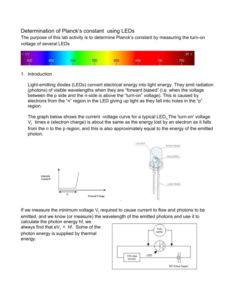
Determination of Planck’s constant using LEDs
The purpose of this lab activity is to determine Planck’s constant by measuring the turn-on
voltage of several LEDs
1. Introduction
Light-emitting diodes (LEDs) convert electrical energy into light energy. They emit radiation
(photons) of visible wavelengths when they are “forward biased” (i.e. when the voltage
between the p side and the n-side is above the “turn-on” voltage). This is caused by
electrons from the “n” region in the LED giving up light as they fall into holes in the “p”
region.
The graph below shows the current -voltage curve for a typical LED. The 'turn-on' voltage
Vt times e (electron charge) is about the same as the energy lost by an electron as it falls
from the n to the p region, and this is also approximately equal to the energy of the emitted
photon.
.
If we measure the minimum voltage Vt required to cause current to flow and photons to be
emitted, and we know (or measure) the wavelength of the emitted photons and use it to
calculate the photon energy hf, we
always find that eVt < hf. Some of the
photon energy is supplied by thermal
energy.
2. Procedure:
Light-emitting diodes require a series load resistor to prevent thermal runaway - unlimited
forward current - from destroying them. Our experiment is conceptually as shown above,
with some modification: we use AC voltage rather than DC, so the voltage keeps varying
periodically, and the LED lights up whenever the voltage is large enough to overcome the
depletion barrier. Then also a current flows across the junction (through the diode). We
measure the applied voltage with an oscilloscope which allows visualization of time
dependent electric signals. We measure the current by measuring the voltage across the
100 resistor. By measuring the voltage Vt at which the LED “turns on”, i.e. at which
current flows (current >0), we can determine the energy of the photons (it is  eVt). This
voltage is different for the LEDs of different color. We know the wavelength of the light
emitted by the different LEDs (and therefore the frequency). By using the equation eV t  hf,
we can determine Planck’s constant h. This is only approximate, since, as mentioned
above, eVt < hf , because some of the energy can be supplied by thermal motion.
A better method is therefore to plot Vt vs frequency and determine the slope of a straight
trendline fitting the data. The slope equals h measured in eV, and the intercept gives an
estimate of the contribution from thermal energy.
3. Analysis
a. Make a table with a row for every LED, containing  (given), f (=c/, c=3108 m/s,
Vt (measured), h (calculated using h (in eV) = Vt /f)
b. Determine mean value of h and standard deviation
c. Graph Vt (on y-axis = ordinate) vs frequency (on x-axis = abscissa) and determine
the slope of the straight line – this is h in units of eV (“electron Volts”)
d. The value of h obtained from the slope of the straight line may be different from that
obtained in part b (from averaging the values of h obtained from different LEDs) –
any explanation? What is the meaning of the intercept? Which of the two
determinations is more reliable?
e.
4. References
http://hyperphysics.phy-astr.gsu.edu/hbase/electronic/led.html#c2
http://micro.magnet.fsu.edu/primer/java/leds/basicoperation/
http://www.youtube.com/watch?v=oVtbWFphcCk
http://www.youtube.com/watch?v=J10QmuB9WCY
5. Information about the LEDs
LED # color
1
2
3
4
5
6
wavelength
(nm)
blue
48040
green
56015
yellow
59015
red
63515
dark red 66515
infrared 95020
max current
(mA)
20
20
20
20
20
20
6. Appendix:
a. More detail about LEDs: A light-emitting diode is a p-n junction rectifier. p-type
material contains excess “holes” (missing electrons – positive) and n-type material
contains excess electrons. When p- and n-type semiconductors are brought together
to form a p-n junction, electrons with energies in the conduction band diffuse from
the n-side to the p-side and holes with energies in the valence band diffuse from the
p-side to the n-side. Without an externally applied voltage, a diffusion potential V D is
generated in the depletion layer between the n-type and the p-type material. The
diffusion potential prevents more electrons and holes from leaving the n- and pregions, respectively, and entering the opposite regions. When an external forward
biased voltage V is applied, the potential barrier is reduced. When V ~ VD the height
of the barrier is approximately zero and electrons can flow from the n-side to the pside, and a current will flow across the junction from the p-type to the n-type
material. As the current flows electrons are continually meeting holes in the p-n
interface. When an electron drops in to a hole level a photon is released with energy
E=hf. The frequency or wavelength of light (color) will depend on the semiconductor
material and diffusion voltage VD. The diode will turn on when V= VD. During the
recombination energy is released. It can be released in the form of a photon with
energy hf ~ Eg, where Eg is the width of the band gap of the semiconductor, which in
turn is  eVD  eVt . The LED junction must be thin and/or transparent so the emitted
light can escape.
b. Use of Excel for this experiment
You should use a spreadsheet program (e.g. Excel) to do the data analysis.
Excel hints:
i.
Getting average and standard deviation: In Excel you can get the average
using the function AVERAGE(data range), and standard deviation by using
function STDEV(data range)
ii. Scatter plot: it is useful to have two columns adjacent to each other, first
column f, then column Vt . Select the data in these two columns and then do
“insert scatter” – this will generate a scatter plot of Vt (y‐axis) vs f (x‐axis).
Then right‐click on data points in chart and select “add trendline”. In the
pop‐up menu, select “linear”, “display equation on chart” and “display R‐value
on chart”
iii. Parameters of trendline: If you want to use the slope from the linear trendline
in calculations (e.g. get h from slope), select an appropriate cell in your
spreadsheet and type =slope(y‐value range, x‐value range). This will put the
slope of the line into the cell. You can also get h directly, typing
=slope(y‐value range, x‐value range) Similarly you could also get the intercept
by typing “= intercept(y‐value range, x‐value range)”
Explanation about average, standard deviation, uncertainties:
(1) if you repeat measurements of the same quantity several times, in general you will see
that the results vary from one attempt to the other; this is due to measurement errors.
Repetition of measurements can be used to get a more precise estimate of the “true
value” and also give information about the measurement precision.
(2) if you have N measurements Xi (i=1,2,…N) of some quantity X, the average value is
1 N
given by
X   Xi
N i 1
(this means: sum all the values Xi, i.e. take X1 + X2 +….+XN, and then divide by the total
number of measurements, N).
(3) the “standard deviation” is a quantity which provides an estimate for the precision with
which you determined your best estimate of X. The square of the standard deviation
(also called the “sample variance”) is given by
1 N
X2 
( X i  X )2 ,

N  1 i 1
i.e. to calculate it, you take the sum of the squares of the deviations between the
individual measurements Xi and the average, and then divide by (N‐1). The standard
deviation (sometimes also called the “root‐mean‐squared deviation”) is then given by
1 N
 ( X i  X )2 .
N  1 i 1
In Excel, you can get the standard deviation by using the function STDEV(data range).
the square root of this:
X 
(4) You can also try to estimate your measurement precision by making an educated
guess (“guesstimate”) of how precisely you know the voltage and the frequency . Let
V   V be the uncertainty (“error”, “imprecision”) of your measurement of the turn-on
voltage Vt , and  f   f the uncertainty of the frequency, then the “relative uncertainty”
h h

of h determined from this is:
h
h
h
h

h
h

V
V
 (
V
V
)2  (
f
f
)2