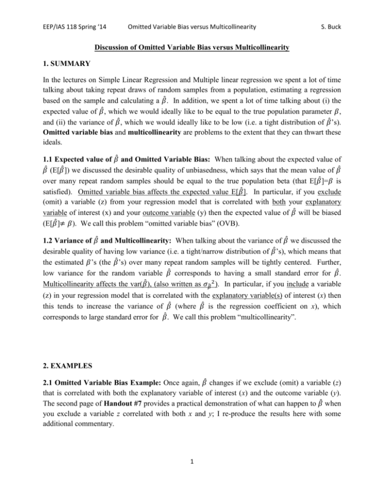
EEP/IAS 118 Spring ‘14
Omitted Variable Bias versus Multicollinearity
S. Buck
Discussion of Omitted Variable Bias versus Multicollinearity
1. SUMMARY
In the lectures on Simple Linear Regression and Multiple linear regression we spent a lot of time
talking about taking repeat draws of random samples from a population, estimating a regression
based on the sample and calculating a 𝛽̂ . In addition, we spent a lot of time talking about (i) the
expected value of 𝛽̂ , which we would ideally like to be equal to the true population parameter 𝛽,
and (ii) the variance of 𝛽̂ , which we would ideally like to be low (i.e. a tight distribution of 𝛽̂ ’s).
Omitted variable bias and multicollinearity are problems to the extent that they can thwart these
ideals.
1.1 Expected value of 𝛽̂ and Omitted Variable Bias: When talking about the expected value of
𝛽̂ (E[𝛽̂ ]) we discussed the desirable quality of unbiasedness, which says that the mean value of 𝛽̂
over many repeat random samples should be equal to the true population beta (that E[𝛽̂ ]=𝛽 is
satisfied). Omitted variable bias affects the expected value E[𝛽̂ ]. In particular, if you exclude
(omit) a variable (z) from your regression model that is correlated with both your explanatory
variable of interest (x) and your outcome variable (y) then the expected value of 𝛽̂ will be biased
(E[𝛽̂ ]≠ 𝛽). We call this problem “omitted variable bias” (OVB).
1.2 Variance of 𝛽̂ and Multicollinearity: When talking about the variance of 𝛽̂ we discussed the
desirable quality of having low variance (i.e. a tight/narrow distribution of 𝛽̂ ’s), which means that
the estimated 𝛽’s (the 𝛽̂ ’s) over many repeat random samples will be tightly centered. Further,
low variance for the random variable 𝛽̂ corresponds to having a small standard error for 𝛽̂ .
Multicollinearity affects the var(𝛽̂ ), (also written as 𝜎𝛽̂ 2 ). In particular, if you include a variable
(z) in your regression model that is correlated with the explanatory variable(s) of interest (x) then
this tends to increase the variance of 𝛽̂ (where 𝛽̂ is the regression coefficient on x), which
corresponds to large standard error for 𝛽̂ . We call this problem “multicollinearity”.
2. EXAMPLES
2.1 Omitted Variable Bias Example: Once again, 𝛽̂ changes if we exclude (omit) a variable (z)
that is correlated with both the explanatory variable of interest (x) and the outcome variable (y).
The second page of Handout #7 provides a practical demonstration of what can happen to 𝛽̂ when
you exclude a variable z correlated with both x and y; I re-produce the results here with some
additional commentary.
1
EEP/IAS 118 Spring ‘14
Omitted Variable Bias versus Multicollinearity
S. Buck
From Handout #7:
Omitting an important variable correlated with the other independent variables:
Omitted variable bias
= 1.17 + .106 educ
(.08) (.005)
+.011 exp
(.0009)
- .26 female
(.02)
+ .012 profocc
(.03)
R2 = .28
n = 2000
= 2.57 +
(.03)
+.011 exp
(.0009)
- .26 female
(.02)
+ .358 profocc
(.03)
R2 = .16
n = 2000
Additional Commentary on Handout #7: The difference between these regression models is that the
second model excludes ‘educ’. As indicated, in the second equation we have excluded (omitted) the
variable ‘educ’ which is an important variable in that it determines the outcome (i.e. education is
correlated with log(wages)); ‘educ’ is also correlated with other explanatory variables, in particular,
the indicator for whether your employment type is a professional occupation (‘profocc’). These
correlations are demonstrated in the correlation matrix below. The correlation between ‘educ’ and
‘lwage’ is 0.4097 (positive) and the correlation between ‘educ’ and ‘profocc’ is 0.4276 (positive).
As a consequence, in the second equation the regression coefficient on ‘profocc’ is measuring the
effect of both having higher education and having a professional occupation; that is, the regression
coefficient on ‘profocc’ exhibits a bias relative to the first equation. Consistent with demonstrations
from class, the bias present in the regression coefficient on ‘profocc’ in the second equation (0.358)
is positive relative to the first equation. Said differently, due to the exclusion of ‘educ’ the
regression coefficient on ‘profocc’ in the second equation is positively biased relative to the first
equation.
. correlate lwage educ exp female profocc nonwhite
(obs=2000)
|
lwage
educ
exper
female profocc nonwhite
-------------+-----------------------------------------------------lwage |
1.0000
educ |
0.4097
1.0000
exper |
0.2358
0.0010
1.0000
female | -0.1935
0.0489
0.0210
1.0000
profocc |
0.2181
0.4276 -0.0383
0.1077
1.0000
nonwhite | -0.0379 -0.0051 -0.0200
0.0368 -0.0143
1.0000
2.2 Multicollinearity Example: As we add variables to our regression model that are correlated
with the explanatory variable(s) of interest, then the standard errors for the 𝛽̂ ’s on the explanatory
variable(s) of interest will increase. The first page of Handout #8 provides a practical
demonstration of what happens to the standard errors for your 𝛽̂ ’s when you include a variable
that is highly correlated with the explanatory variables already in the model; I re-produce the
relevant results from Handout #8 here with some additional commentary.
2
EEP/IAS 118 Spring ‘14
Omitted Variable Bias versus Multicollinearity
S. Buck
From Handout #8:
(1) None
. reg lwage educ exper female
Source |
SS
df
MS
-------------+-----------------------------Model |
182.35726
3 60.7857535
Residual | 490.219607 1996 .245601005
-------------+-----------------------------Total | 672.576867 1999 .336456662
Number of obs
F( 3, 1996)
Prob > F
R-squared
Adj R-squared
Root MSE
=
=
=
=
=
=
2000
247.50
0.0000
0.2711
0.2700
.49558
-----------------------------------------------------------------------------lwage |
Coef.
Std. Err.
t
P>|t|
[95% Conf. Interval]
-------------+---------------------------------------------------------------educ |
.1167441
.0053157
21.96
0.000
.1063191
.127169
exper |
.0109089
.000869
12.55
0.000
.0092046
.0126132
female | -.2543189
.0222067
-11.45
0.000
-.2978696
-.2107682
_cons |
1.055792
.0757381
13.94
0.000
.9072576
1.204326
------------------------------------------------------------------------------
(1) Almost collinear
. reg lwage educ exper female age
Source |
SS
df
MS
-------------+-----------------------------Model | 182.468262
4 45.6170655
Residual | 490.108605 1995 .245668474
-------------+-----------------------------Total | 672.576867 1999 .336456662
Number of obs
F( 4, 1995)
Prob > F
R-squared
Adj R-squared
Root MSE
=
=
=
=
=
=
2000
185.69
0.0000
0.2713
0.2698
.49565
-----------------------------------------------------------------------------lwage |
Coef.
Std. Err.
t
P>|t|
[95% Conf. Interval]
-------------+---------------------------------------------------------------educ |
.1692465
.1115687
1.52
0.129
-.0495568
.3880498
exper |
.0633711
.1113346
0.57
0.569
-.1549732
.2817154
female | -.2545469
.0222135
-11.46
0.000
-.298111
-.2109827
age | -.0524796
.1113744
-0.47
0.638
-.270902
.1659428
_cons |
1.370917
.6728026
2.04
0.042
.0514472
2.690386
------------------------------------------------------------------------------
Commentary on example from Handout #8: The difference between these regression models is
that the second model includes the variable ‘age’. In the first set of regression results we see
relatively small standard errors for the 𝛽̂ ’s on ‘educ’ and ‘exper’ as indicated by numbers reported
in the column under ‘Std. Err.’. In the second set of regression results we see that standard errors
for these two 𝛽̂ ’s are considerably larger. Why does this happen? If the variable added to the
regression equation (e.g. age) is highly correlated with variables already in the model (e.g. educ
and exper), then standard errors for the associated 𝛽̂ will get very large. This is what is meant by
multicollinearity. We are concerned about multicollinearity because large standard errors for the
𝛽̂ ’s produce large confidence intervals and makes it likely that you will fail to reject the null
hypothesis even if the magnitude of the estimated regression coefficient (𝛽̂ ) is much different than
the null hypothesis. Note: The heading “None” on the first set of regression results reflects the
3
EEP/IAS 118 Spring ‘14
Omitted Variable Bias versus Multicollinearity
S. Buck
fact that the standard errors are small, which suggests that the variables in the model are not close
to being collinear (i.e. they are not close to being perfectly correlated). The heading “Almost
collinear” for the second set of regression results reflects the fact that the standard errors are very
large, which suggest that some of the variables are very highly correlated (i.e. they are almost
collinear/perfectly correlated).
3. INTERPRETATION: Question 2 on Quiz #1
The T/F question on Quiz #1 was designed to help illustrate the difference between the problem of
omitted variable bias and multicollinearity before exam time. I know the question was a difficult
one for many of you so it is a good idea to re-visit the problem. As the discussion above suggests,
good ways to distinguish between Omitted Variable Bias and Multicollinearity are:



Omitted variable bias affects the E[𝛽̂ ], while multicollinearity affects the var[𝛽̂ ].
Omitted variable bias can occur when you exclude an additional variable (z) from your
regression model, while multicollinearity can occur when you include an additional
variable.
Omitted variable bias is problematic when an excluded (omitted) variable z is correlated
with both the explanatory variable of interest and the outcome variable, while
multicollinearity can be introduced if an included variable z is correlated with just the
explanatory variable of interest (x) regardless of whether the included variable z is
correlated with the outcome variable (y).
Having summarized these distinguishing characteristics, let’s revisit the question on
multicollinearity from Quiz #1 which I re-produce:
Multicollinearity in a multiple linear regression model arises when you add covariates
(explanatory variables) to the regression model that are highly correlated with the
explanatory variable of interest.
T/F When adding covariates to your multiple linear regression model that are highly
correlated with the explanatory variable of interest, this multicollinearity is a cause for
concern because it biases the beta coefficient on the explanatory variable of interest. Justify
your answer in a sentence or two (i.e.: if you answer true or false, explain why the answer
is true or false).
Response: You already have the solution so I won’t reproduce that here. However, I wanted to
make explicit the clues that should have signaled to you that something was wrong with the
statement. The statement clearly indicates that we are adding variables to our model—this would
not introduce omitted variable bias, because that happens when we exclude variables from the
model, not include variables. Second, the concept of multicollinearity relates to a high degree of
correlation between just explanatory variables and how this affects the variance of the betas, not
bias in the regression coefficients (𝛽̂ ’s) themselves.
4