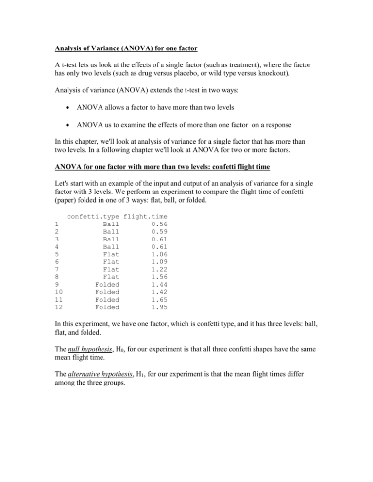
Analysis of Variance (ANOVA) for one factor
A t-test lets us look at the effects of a single factor (such as treatment), where the factor
has only two levels (such as drug versus placebo, or wild type versus knockout).
Analysis of variance (ANOVA) extends the t-test in two ways:

ANOVA allows a factor to have more than two levels

ANOVA us to examine the effects of more than one factor on a response
In this chapter, we'll look at analysis of variance for a single factor that has more than
two levels. In a following chapter we'll look at ANOVA for two or more factors.
ANOVA for one factor with more than two levels: confetti flight time
Let's start with an example of the input and output of an analysis of variance for a single
factor with 3 levels. We perform an experiment to compare the flight time of confetti
(paper) folded in one of 3 ways: flat, ball, or folded.
1
2
3
4
5
6
7
8
9
10
11
12
confetti.type flight.time
Ball
0.56
Ball
0.59
Ball
0.61
Ball
0.61
Flat
1.06
Flat
1.09
Flat
1.22
Flat
1.56
Folded
1.44
Folded
1.42
Folded
1.65
Folded
1.95
In this experiment, we have one factor, which is confetti type, and it has three levels: ball,
flat, and folded.
The null hypothesis, H0, for our experiment is that all three confetti shapes have the same
mean flight time.
The alternative hypothesis, H1, for our experiment is that the mean flight times differ
among the three groups.
Here's the output from the ANOVA, which we'll look at in more detail shortly.
Analysis of Variance Table
Response: flight.time
Df Sum Sq Mean Sq F value
Pr(>F)
confetti.type 2 2.13522 1.06761 28.157 0.0001338 ***
Residuals
9 0.34125 0.03792
--Signif. codes: 0 ‘***’ 0.001 ‘**’ 0.01 ‘*’ 0.05 ‘.’ 0.1 ‘ ’ 1
The ANOVA p-value for the factor confetti type is 0.0001338. The p-value is less than
0.05, so we reject the null hypothesis and conclude that at least one of the three confetti
types has a different mean flight time from the other two types. When we look at the
graph this result is plausible.
Example of ANOVA for one factor with more than two levels: chick weight
An experiment was conducted to measure and compare the effectiveness of various feed
supplements on the growth rate of chickens (Anonymous (1948) Biometrika, 35, 214).
Newly hatched chicks were randomly allocated into six groups, and each group was
given a different feed supplement. Their weights in grams after six weeks are given along
with feed types.
Chick weight in grams
horsebean
179
160
136
227
217
168
108
124
143
140
linseed
309
229
181
141
260
203
148
169
213
257
244
271
soybean
243
230
248
327
329
250
193
271
316
267
199
171
sunflower
423
340
392
339
341
226
320
295
334
322
297
318
meatmeal
325
257
303
315
380
153
263
242
206
344
258
casein
368
390
379
260
404
318
352
359
216
222
283
158
248
332
The null hypothesis, H0, for our experiment is that all six treatment groups have the same
mean.
The alternative hypothesis, H1, for our experiment is that the means differ among the six
treatment groups.
In a later section, we'll see how ANOVA calculates a p-value. For now, we'll just look at
the results of the analysis of variance for the chickwt data to see an example of the
output.
Analysis of Variance Table
Response: weight
Df Sum Sq Mean Sq F value
Pr(>F)
feed
5 231129
46226 15.365 5.936e-10 ***
Residuals 65 195556
3009
The ANOVA p-value for the factor "feed" is 5.936e-10. The p-value is less than 0.05, so
we reject the null hypothesis, and conclude that at least one of the six treatment groups
has a mean different from the other groups. When we look at the graph of the weights
versus feed type, this result is plausible. Always check graphs of your data to make sure
the statistical analysis has been done correctly and makes sense.
How ANOVA calculates a p-value
Back in my garden, I'd like to increase the number of flowers that my roses produce. I
think that giving them more water may increase the number of flowers. I'll have three
treatment groups with 10 roses each:



0 gallons extra per week (control group)
1 gallon extra per week
2 gallons extra per week
From the 200 rose plants in my garden, I randomly select 30 roses for my experiment,
and randomly assign 10 rose plants to each treatment group. At the end of one month I'll
count the number of flowers produced by each plant.
Suppose that, unfortunately, the null hypothesis is true: the extra water has no effect on
the number of roses. Figure <roses> shows the distribution of the number of flowers on
all 200 plants. The 10 roses in each of the three treatment groups are shown with different
symbols.
Here are the numbers of flowers on the roses in each treatment group, and the treatment
group means.
Treatment
(gallons)
0
1
2
N
Number of flowers on
each rose
10 14, 15, 18, 19, 21, 21, 23,
27, 28, 28
10 6, 13, 19, 20, 20, 20, 21,
23, 27, 27
10 7, 8, 15, 16, 19, 20, 21,
21, 21, 26
Treatment group
mean
21.4
Standard
deviation
5.10
19.6
6.26
17.4
6.02
We see that the means of the three treatment groups are different. When we do an actual
experiment, we don't know if the null hypothesis is true. So we have to ask, what is the
probability that the observed differences in means would have occurred if the null
hypothesis is true? Can the observed differences in means be explained by random
variation in sampling from a single population?
When we look at the plot of the number of flowers versus the number of gallons of water,
we see little evidence that the amount of water has any effect. The variation within each
treatment group is large compared to the difference between the groups.
How can we calculate the probability that the observed results, or more extreme results,
would have occurred if the null hypothesis was true? You might think of doing pairwise
t-tests to compare 0 versus 1 gallon, 0 versus 2 gallons, and 1 versus 2 gallons. As we'll
see shortly, the method of doing all possible pairwise t-tests (doing multiple
comparisons) increases the risk of a false discovery. The risk of false discovery increases
with the number of treatment groups we compare. So we'd like a single test that tells us if
any of the treatment groups are different.
Recall that when we developed the t-test, we used the ratio:
Mean ( placebo )  Mean (drug )
Error in estimating the difference
We calculated the T statistic:
T=
Mean( placebo )  Mean(drug )
SEM ( placebo ) 2  SEM (drug ) 2
The denominator of the T statistics uses the standard error of the mean:
Standard Error of the Mean = SEM = 𝑆𝑥̅
= (Sample standard deviation)/(Square root of N)
s
=
N
So the standard error of the mean is large when the standard deviation within treatment
group, s, is large. When T is large, the difference between the means of the treatment
groups is large compared to the variability within treatment group. This is the same
concept as for ANOVA: the difference between the means of the treatment groups is
large compared to the variability within treatment group.
But we need to modify the T statistic ratio so we can have more than two treatment
groups. For ANOVA, we'll re-cast the ratio:
Mean ( placebo )  Mean (drug )
Error in estimating the difference
as
𝑉𝑎𝑟𝑖𝑎𝑏𝑖𝑙𝑖𝑡𝑦 𝑎𝑚𝑜𝑛𝑔 (𝑜𝑟 𝑏𝑒𝑡𝑤𝑒𝑒𝑛) 𝑡ℎ𝑒 𝑡𝑟𝑒𝑎𝑡𝑚𝑒𝑛𝑡 𝑔𝑟𝑜𝑢𝑝𝑠 𝑚𝑒𝑎𝑛𝑠
𝑉𝑎𝑟𝑖𝑎𝑏𝑖𝑙𝑖𝑡𝑦 𝑤𝑖𝑡ℎ𝑖𝑛 𝑡ℎ𝑒 𝑡𝑟𝑒𝑎𝑡𝑚𝑒𝑛𝑡 𝑔𝑟𝑜𝑢𝑝𝑠
When this ratio is large, we have evidence that the treatments differ: the differences
among the treatment groups means are large compared to the within group variance.
When this ratio is small, evidence indicates that the treatments do not differ: the
differences among the treatment groups means are small compared to the within group
variance.
Now let's see how we can calculate a single number to represent our ratio. Let's start with
the denominator, the variability within the treatment groups. When the null hypothesis is
true, we can describe the variability within the treatment groups using the variance (or
standard deviation) of the observations within each treatment group. The average of these
within-group variances is a good estimate of the population variance. We'll calculate this
average, and call it the within group estimate of the population variance.
For our example using flowers on roses, we have the following within-group variance.
Within-group variance = average [(variance of 0 gallon group) + (variance of 1 gallon
group) + (variance of 2 gallon group)]
Within-group variance =
2
𝑠𝑤𝑖𝑡ℎ𝑖𝑛
=
1 2
(𝑠
+ 𝑠12 𝑔𝑎𝑙𝑙𝑜𝑛 + 𝑠22 𝑔𝑎𝑙𝑙𝑜𝑛 )
3 0 𝑔𝑎𝑙𝑙𝑜𝑛
= (5.1033762 + 6.25742 + 6.0221812)/3
= 33.822
2
So our estimate of the population variance, 𝑠𝑤𝑖𝑡ℎ𝑖𝑛
, based on the within-group sample
variance, is 33.822.
Next, let's look at the numerator of the ratio, the varability among (or between) the
treatment groups means. For the t-test, the numerator was the difference between the two
treatment groups means. For ANOVA, where we can have three or more treatment
groups, we don't want to calculate all pairwise differences between the means. That
method would give us many numbers, instead of just one number to use in the ratio. We
want a single number that describes the variability of the treatment group means. One
such number is the standard deviation of the treatment group means 𝑆𝑥̅ .
For our example using flowers on roses when the null hypothesis is true, we have the
following standard deviation of the treatment group means 𝑆𝑥̅ .
First, we calculate the grand mean of the k = 3 treatment group means.
Grand mean of the three treatment group means:
𝑋̅𝑥̅ = average [(mean of 0 gallon group) + (mean of 1 gallon group) + (mean of 2 gallon
group)]
𝑋̅𝑥̅ =
1
3
(𝑋̅ 0 𝑔𝑎𝑙𝑙𝑜𝑛 + 𝑋̅ 1 𝑔𝑎𝑙𝑙𝑜𝑛 + 𝑋̅ 2 𝑔𝑎𝑙𝑙𝑜𝑛 ) =
1
3
(21.4 + 39.6 + 37.4) = 32.8
2
2
2
̅ 0 𝑔𝑎𝑙𝑙𝑜𝑛 − 𝑋̅𝑥̅ ) + (𝑋̅ 1 𝑔𝑎𝑙𝑙𝑜𝑛 − 𝑋̅𝑥̅ ) + (𝑋̅ 2 𝑔𝑎𝑙𝑙𝑜𝑛 − 𝑋̅𝑥̅ )
𝑋
(
𝑆𝑥̅ = √
𝑘−1
(21.4 − 32.8)2 + (39.6 − 32.8)2 + (37.4 − 32.8)2
𝑆𝑥̅ = √
3−1
𝑆𝑥̅ = 2.033
We have the standard deviation of the 3 treatment group means 𝑆𝑥̅ , = 2.033. Recall that
the standard deviation of the treatment group means, 𝑆𝑥̅ , has a special name, the
Standard Error of the Mean, and is defined as follows.
𝑆𝑥̅ = (Sample standard deviation)/(Square root of N)
s
=
N
We can use this formula and the observed values of 𝑆𝑥̅ , = 2.033 and N = 10 (for the 10
roses in each treatment group) to get a second estimate of the population variance. This
estimate is based on the variability of the treatment means.
2
2
𝑠𝑏𝑒𝑡𝑤𝑒𝑒𝑛
= 𝑁 𝑆𝑥̅ = 10 ∗ 2.033 = 40.133
Recall the ratio we wanted:
𝑉𝑎𝑟𝑖𝑎𝑏𝑖𝑙𝑖𝑡𝑦 𝑎𝑚𝑜𝑛𝑔 (𝑜𝑟 𝑏𝑒𝑡𝑤𝑒𝑒𝑛) 𝑡ℎ𝑒 𝑡𝑟𝑒𝑎𝑡𝑚𝑒𝑛𝑡 𝑔𝑟𝑜𝑢𝑝𝑠 𝑚𝑒𝑎𝑛𝑠
𝑉𝑎𝑟𝑖𝑎𝑏𝑖𝑙𝑖𝑡𝑦 𝑤𝑖𝑡ℎ𝑖𝑛 𝑡ℎ𝑒 𝑡𝑟𝑒𝑎𝑡𝑚𝑒𝑛𝑡 𝑔𝑟𝑜𝑢𝑝𝑠
If the amount of water has no effect, the population variance estimated using the
numerator (variability among the treatment means) should be approximately equal to the
population variance estimated using the denominator, (variability with treatment groups).
We'll call this ratio the F statistic.
𝐹=
𝑠2𝑏𝑒𝑡𝑤𝑒𝑒𝑛
2
𝑠𝑤𝑖𝑡ℎ𝑖𝑛
=
40.133
33.822
= 1.1866
Is the value of F = 1.1866 large enough to indicate a significant effect of water? Or would
we see an F statistic this large just by random variation of sampling, when water has no
effect? More specifically, what is the probability that we would observe an F-statistic of
1.1866 or larger if the null hypothesis is true?
Recall that previously, when we wanted to calculate a p-value, we used a permutation
test. We randomly permuted (shuffled) the treatment group identifiers several hundred or
thousand times. Each time, we calculated the difference between the means of the two
treatment groups. Finally, we asked what proportion of the random permutations gave a tstatistics as large or larger than the t-statistic observed in our actual experiment. We can
apply the same permutation method to ANOVA. The only change is that now we can
have two or more treatment groups. When we randomly shuffle, we shuffle the labels
among observations in all the treatment groups.
Here are the F-statistic values from 1000 random shuffles of the rose flower data. What
proportion of these 1000 random shuffles give an F-statistic larger than the F-statistic
observed in our experiment. F=1.1866? Of the 1000 random shuffles, there are 331 with
an F-statistic greater than or equal to 1.1866. So the probability that we would observe an
F-statistic greater than or equal to 1.1866 is 331/1000 or p=0.331. This p-value is much
greater than the usual threshold of alpha = 0.05. This result tells us that an F-statistic of
1.1866 can occur by random variation much more than 5 percent of the time.
We could use the permutation method to calculate p-values for all our analyses.
However, the distribution of the F values is very reproducible, and statisticians have
found a formula that gives values very similar to what we get using the permutation
method. The advantage of the formula is that it is easy to calculate, and doesn't require
doing permutations, which were laborious before computers were invented. The
distribution of F-value is called the F distribution. The shape of the F distribution
depends on (i) the number of treatment groups and (ii) the number of observations within
each treatment group.
Here is the output when we analyze the rose data set using a statistics software package
that uses the formula for the F-distribution.
.
Analysis of Variance Table
Response: Flowers
Df Sum Sq Mean Sq F value Pr(>F)
factor(Water) 2 80.27 40.133 1.1866 0.3207
Residuals
27 913.20 33.822
Let's compare the ANOVA table to the calculations we did above. We calculated the F
statistic:
𝐹=
𝑠2𝑏𝑒𝑡𝑤𝑒𝑒𝑛
2
𝑠𝑤𝑖𝑡ℎ𝑖𝑛
=
40.133
33.822
= 1.1866
These are the same values that we see in the ANOVA table.
We used random permutations to determine the p-value for this data set. We'll get a
slightly different p-value each time, because of the random permutations. Analyzing the
rose data set using a statistics software package that uses the formula for the Fdistribution, we get a p-value of 0.3207. This p-value is quite close to the p-value of
p=0.331 using 1000 permutations. We can do more permutations, say, 10,000 to increase
the accuracy.
Example ANOVA calculations when more water increases the number of flowers
Now let's look at our example using flowers on roses when the null hypothesis is false.
Suppose that either 1 or 2 gallons of water increases the number of flowers on each plant
by 20. We get the following results.
Number of flowers versus treatment group when 1 or 2 gallons of water increases the
number of flowers on each plant.
Treatment
N Number of flowers on
Treatment group
Standard
(gallons)
each rose
mean
deviation
0
10 0, 2, 4
2
2
1
10 4, 6, 8
6
2
2
10 6, 8, 10
8
2
With this new data, the differences between the means of the treatment group is large
compared to the variation within each treatment group. This is much more convincing
evidence that the amount of water has an effect on the number of flowers.
We have the following within-group variance.
Within-group variance = average [(variance of 0 gallon group) + (variance of 1 gallon
group) + (variance of 2 gallon group)]
Within-group variance =
2
𝑠𝑤𝑖𝑡ℎ𝑖𝑛
=
1 2
(𝑠
+ 𝑠12 𝑔𝑎𝑙𝑙𝑜𝑛 + 𝑠22 𝑔𝑎𝑙𝑙𝑜𝑛 )
3 0 𝑔𝑎𝑙𝑙𝑜𝑛
= (22 + 22+ 22)/3
=4
2
So our estimate of the population variance, 𝑠𝑤𝑖𝑡ℎ𝑖𝑛
, based on the within-group sample
variance, is 4.
Next, the varability among (or between) the treatment groups means. The grand mean of
the three treatment group means:
𝑋̅𝑥̅ = average [(mean of 0 gallon group) + (mean of 1 gallon group) + (mean of 2 gallon
group)]
𝑋̅𝑥̅ =
1
3
(𝑋̅ 0 𝑔𝑎𝑙𝑙𝑜𝑛 + 𝑋̅ 1 𝑔𝑎𝑙𝑙𝑜𝑛 + 𝑋̅ 2 𝑔𝑎𝑙𝑙𝑜𝑛 ) =
1
3
(2 + 6 + 8) = 5.33
2
2
2
̅ 0 𝑔𝑎𝑙𝑙𝑜𝑛 − 𝑋̅𝑥̅ ) + (𝑋̅ 1 𝑔𝑎𝑙𝑙𝑜𝑛 − 𝑋̅𝑥̅ ) + (𝑋̅ 2 𝑔𝑎𝑙𝑙𝑜𝑛 − 𝑋̅𝑥̅ )
𝑋
(
𝑆𝑥̅ = √
𝑘−1
(2 − 5.33)2 + (6 − 5.33)2 + (8 − 5.33)2
𝑆𝑥̅ = √
3−1
𝑆𝑥̅ = 3.055
We know 𝑆𝑥̅ = (Sample standard deviation)/(Square root of N)
s
=
N
We use this formula to estimate the population variance. This estimate is based on the
variability of the treatment means.
2
2
𝑠𝑏𝑒𝑡𝑤𝑒𝑒𝑛
= 𝑁 𝑆𝑥̅ = 10 ∗ 3.055 = 28
Recall the ratio we wanted:
𝑉𝑎𝑟𝑖𝑎𝑏𝑖𝑙𝑖𝑡𝑦 𝑎𝑚𝑜𝑛𝑔 (𝑜𝑟 𝑏𝑒𝑡𝑤𝑒𝑒𝑛) 𝑡ℎ𝑒 𝑡𝑟𝑒𝑎𝑡𝑚𝑒𝑛𝑡 𝑔𝑟𝑜𝑢𝑝𝑠 𝑚𝑒𝑎𝑛𝑠
𝑉𝑎𝑟𝑖𝑎𝑏𝑖𝑙𝑖𝑡𝑦 𝑤𝑖𝑡ℎ𝑖𝑛 𝑡ℎ𝑒 𝑡𝑟𝑒𝑎𝑡𝑚𝑒𝑛𝑡 𝑔𝑟𝑜𝑢𝑝𝑠
If the amount of water has no effect, the population variance estimated using the
numerator (variability among the treatment means) should be approximately equal to the
population variance estimated using the denominator, (variability with treatment groups).
We'll call this ratio the F statistic.
2
𝐹=
𝑠𝑏𝑒𝑡𝑤𝑒𝑒𝑛
2
𝑠𝑤𝑖𝑡ℎ𝑖𝑛
=
28
4
=7
Is the value of F = 7 large enough to indicate a significant effect of water? Or would we
see an F statistic this large just by random variation of sampling, when water has no
effect? More specifically, what is the probability that we would observe an F-statistic of 7
or larger if the null hypothesis is true?
The typical output from software is an ANOVA table like this.
Response: Flowers
Df Sum Sq Mean Sq F value Pr(>F)
factor(Water) 2
56
28
7 0.027 *
Residuals
6
24
4
The ANOVA software gives p=0.027 for the factor water. So we reject the null
hypothesis and conclude that more water does have an effect on the number of flowers.
Notice that the ANOVA table also provides the F-statistics value (7). The column labeled
2
"Mean Sq" in the ANOVA table gives the population variance 𝑠𝑏𝑒𝑡𝑤𝑒𝑒𝑛
based on the
2
treatment group means, which is 28, and the population variance, 𝑠𝑤𝑖𝑡ℎ𝑖𝑛 , based on the
within-group sample variance, which is 4.
Which groups are different?
After doing the ANOVA, a significant p-value tells us that at least one of the groups is
different from the other groups. However, it doesn’t tell us which group or groups are
different. One way to see which treatment groups are different is to do pairwise t-tests
among all pairs of treatments. If we do all possible pairwise contrasts of groups, we could
do a large number of tests, and increase the risk of a type I error (false positive) just
because of the multiple comparisons we perform. We'll look at this issue shortly.
Treatment contrasts
For treatment contrasts, one group is chosen as the baseline group and all other groups
are compared to that baseline group. The treatment contrasts give you the actual values of
the differences in means between groups, with no adjustment. Let's look at treatment
contrasts for the chick weight data.
This example uses the summary() function in R to produce the treatment contrasts.
Coefficients:
Estimate Std. Error t value Pr(>|t|)
(Intercept)
323.583
15.834 20.436 < 2e-16 ***
feedhorsebean -163.383
23.485 -6.957 2.07e-09 ***
feedlinseed
-104.833
22.393 -4.682 1.49e-05 ***
feedmeatmeal
-46.674
22.896 -2.039 0.045567 *
feedsoybean
-77.155
21.578 -3.576 0.000665 ***
feedsunflower
5.333
22.393
0.238 0.812495




Estimate = the regression coefficients
Std. Error = the standard error of the regression coefficients
t value = the T statistic = Estimate/Std. Error
Pr(>|t|) = the probability that the T statistic would be as large as observed if the
null hypothesis were true.
The interpretation of these estimates is that the first line in the ANOVA table for the
intercept is the mean of the first group (casein), which is 323.583.
(Intercept)
Estimate Std. Error t value Pr(>|t|)
323.583
15.834 20.436 < 2e-16 ***
The second line (feedhorsebean) third line (feedlinseed) and so on in the ANOVA
table describe the difference between those groups and the first group.
So the second line (feedhorsebean) has an estimate of -163.383, indicating that the
mean for (feedhorsebean) is 163.383 less than the mean for casein.
Estimate Std. Error t value Pr(>|t|)
feedhorsebean -163.383
23.485 -6.957 2.07e-09 ***
The third line (feedlinseed) has an estimate of -104.833, indicating that the mean for
(feedlinseed) is 104.833 less than the mean for casein.
feedlinseed
-104.833
22.393
-4.682 1.49e-05 ***
These are so-called "treatment" contrasts, in which the first group is the baseline group
and all other groups are compared to the baseline group.
False positive results: The multiple comparison problem
A problem that arises when you do many comparisons is that, eventually, you will get
some false positive differences just because you have done many comparisons. This is
called the "multiple testing" or "multiple comparison" problem. Suppose that you do two
t-tests, each with alpha (false positive rate) of p=0.05. The probability of a false positive
result when you do two tests is no longer 0.05. The probability of a false positive result
when you do two tests is approximately 0.05 + 0.05 = 0.1. (When the number of tests is
small, the false positive rate is approximately the sum of the alphas for each test.) If you
do three t-tests, the probability of a false positive result is approximately 0.05 + 0.05 +
0.05 = 0.15.
Several methods have been developed to adjust p-values to control for possible false
positive results due to multiple testing. All the methods apply some sort of penalty or
correction to the p-value, to reduce the chance of type I error. Depending on the software
you use, you may have one or more alternative methods. Commonly used methods
include the Bonferroni adjustment, Holm's test, Tukey's test, and Fisher's Least
Significant Difference. If you are comparing several treatments against a single control
(rather than all possible pairwise comparisons), then Dunnett's test is a good choice.
Bonferroni correction
The most conservative method is the Bonferroni correction. If you use Bonferroni, you
won't get many false positives, but you will get a lot of false negative results. The
Bonferroni method gives you very little power to detect real relationships. Alternative
methods are less conservative, and give you more power.
Divide the target alpha (typically alpha=0.05 or 0.01) by the number of tests being
performed. If the unadjusted p-value is less than the Bonferroni-corrected target alpha,
then reject the null hypothesis. If the unadjusted p-value is greater than the Bonferronicorrected target alpha, then do not reject the null hypothesis.
Example of Bonferroni correction.
Suppose we have k = 3 t-tests. The unadjusted p-values are
p1 = 0.001
p2 = 0.013
p3 = 0.074
Assume alpha = 0.05. The Bonferroni corrected p-value for significance is alpha/k =
0.05/3 = 0.0167. So the unadjusted p-value must be less than 0.0167 to be significant.
p1 = 0.001 < 0.0167, so reject null
p2 = 0.013 < 0.0167, so reject null
p3 = 0.074 > 0.0167, so do not reject null
Bonferroni adjusted p-values.
An alternative, equivalent way to implement the Bonferroni correction is to multiply the
unadjusted p-value by the number of hypotheses tested, k, up to a maximum Bonferroni
adjusted p-value of 1. If the Bonferroni adjusted p-value is still less than the original
alpha (say, 0.05), then reject the null.
Unadjusted p-values are
p1 = 0.001
p2 = 0.013
p3 = 0.074
Bonferroni adjusted p-values are
p1 = 0.001 * 3 = 0.003
p2 = 0.013 * 3 = 0.039
p3 = 0.074 * 3 = 0.222
Here is the Bonferroni method applied to the chick weight data.
Pairwise comparisons using t tests with pooled SD
data:
chickwts$weight and chickwts$feed
horsebean
linseed
meatmeal
soybean
sunflower
casein
3.1e-08
0.00022
0.68350
0.00998
1.00000
horsebean
0.22833
0.00011
0.00487
1.2e-08
linseed
0.20218
1.00000
9.3e-05
meatmeal
1.00000
0.39653
soybean
0.00447
P value adjustment method: bonferroni
Other multiple comparison correction methods can provide adjusted p-values, though in
general calculation of the adjusted p-value is more complicated than is the case for
Bonferroni.
Holm’s test
For the Bonferroni correction, we apply the same critical value (alpha/k) to all the
hypotheses simultaneously. It is called a “single-step” method.
The Holm’s test is a stepwise method, also called a sequential rejection method, because
it examines each hypothesis in an ordered sequence, and the decision to accept or reject
the null depends on the results of the previous hypothesis tests.
The Holm’s test is less conservative than the Bonferroni correction, and is therefore more
powerful. The Holm’s test uses a stepwise procedure to examine the ordered set of null
hypotheses, beginning with the smallest P value, and continuing until it fails to reject a
null hypothesis.
Example of Holm’s test.
Suppose we have k = 3 t-tests.
Assume target alpha(T)= 0.05.
Unadjusted p-values are
p1 = 0.001
p2 = 0.013
p3 = 0.074
For the jth test, calculate alpha(j) = alpha(T)/(k – j +1)
For test j = 1,
alpha(j) = alpha(T)/(k – j +1)
= 0.05/(3 – 1 + 1)
= 0.05 / 3
= 0.0167
For test j=1, the observed p1 = 0.001 is less than alpha(j) = 0.0167, so we reject the null
hypothesis.
For test j = 2,
alpha(j) = alpha(T)/(k – j +1)
= 0.05/(3 – 2 + 1)
= 0.05 / 2
= 0.025
For test j=2, the observed p2 = 0.013 is less than alpha(j) = 0.025, so we reject the null
hypothesis.
For test j = 3,
alpha(j) = alpha(T)/(k – j +1)
= 0.05/(3 – 3 + 1)
= 0.05 / 1
= 0.05
For test j=3, the observed p2 = 0.074 is greater than alpha(j) = 0.05, so we do not reject
the null hypothesis.
Here are the adjusted p-values using Holm's method for the chick weight data.
horsebean
linseed
meatmeal
soybean
sunflower
casein
2.9e-08
0.00016
0.18227
0.00532
0.81249
horsebean
0.09435
9.0e-05
0.00298
1.2e-08
linseed
0.09435
0.51766
8.1e-05
meatmeal
0.51766
0.13218
soybean
0.00298
P value adjustment method: holm
Calculating the probability of a false positive result with multiple comparisons
It's pretty easy to calculate the probability of a false positive result when we do multiple
comparisons.
P(at least one false positive result) = 1 - P(no false positive results)
For a single T-test, the probability of getting a false positive result is alpha = 0.05.
The probability of not getting a false positive result is 1 – alpha = 1 - 0.05 = 0.95.
If we do k = 2 t-tests, the probability of getting no false positives on any test is 0.95^k =
0.95^2
P(at least one false positive result)
= 1 - P(zero false positive results)
= 1 – (1 - .05) ^ k
= 1 – (1 - .05) ^ 2
= 1 – (.95) ^ 2
= 0.0975
We've increased the risk of a false positive result from p=0.05 for one test, to p=0.0975
doing two tests.
If we do k = 5 t-tests, the probability of getting no false positives on any test is 0.95^k =
0.95^5
P(at least one false positive result)
= 1 - P(zero false positive results)
= 1 – (1 - .05) ^ k
= 1 – (1 - .05) ^ 5
= 1 – (.95) ^ 5
= 0.226
If we do 10 t-tests with alpha = 0.05, then
P(at least one false positive result)
= 1 – (.95) ^ 10
= 0.40
If we do 20 t-tests with alpha = 0.05, then
P(at least one false positive result) =
= 1 – (.95) ^ 20
= 0.64
What if we do 100 t-tests with alpha = 0.05, for 100 genes?
Then P(at least one false positive result)
= 1 – (.95) ^ 100
= 0.994
Gene expression studies use microarrays with 10,000 genes. In genotyping studies, we
may examine the association of 500,000 SNP’s with a disease outcome. In such studies,
the probability of at least one false positive result is virtually certain.
Is the ANOVA model appropriate? Model diagnostics
To give valid results, analysis of variance requires that several assumptions are at least
approximately correct.
1. The observations or data points are independent from all other observations. This
assumption will be violated if some of the observations are correlated. For
example, children in the same family may have correlated scores on IQ; they are
more similar to each other than two children from different families. Mice from
the same litter more be more similar to each other than mice from different litters¸
and have correlated scores on behavior tests. Repeated observations on the same
individual are very likely to be correlated, and should not be treated as though
they were independent measurements.
2. The observations are a representative random sample of the population. Here is an
example of a sample that is not representative. Suppose you want to know the
average weight of fish in an aquarium. You select 5 fish "at random" by catching
5 fish with your fish net. Is it possible that you catch the large, slow moving fish
near the surface, but don't catch the small, fast-moving fish hiding among the
rocks? If so, you do not have a representative random sample of the population,
and your conclusions will not be valid.
3. The population you are sampling from is normally distributed. Many populations
are not normally distributed. Looking at a graph showing the distribution of your
samples is important.
4. The standard deviations of the treatment groups must be the same. This
assumption may be violated if a treatment increases the variance of a treatment
group.
If these assumptions are not met, there are several possible strategies.
1. Correlated observations. You can select one representative of each of set of
correlated observations. This can waste a lot of useful data. Alternatively, you can
use statistical methods that explicitly handle correlated observations. Such
methods are described in the textbooks <correlated data texts>.
2. Non-representative sample of the population. There is not much you can do
except to try to make your sample representative.
3. Non-normal population. You may be able to transform your data so that it is
approximately normal. If that is not possible, you can use a rank method. See the
material on Wilcoxon and Kruskal-Wallis tests in "Alternatives to t-tests and
Anova based on ranks".
4. Unequal standard deviations in treatment groups. You may be able to transform
your data so that the standard deviations are roughly equal. See the chapter on
"Transforming data". If that is not possible, you can use a rank method. See the
material on "Alternatives to t-tests and Anova based on ranks".
We also want to check if there are influential observations and outliers that have a large
effect on the model. If you have such observations, try running your analyses including
and excluding the observations to see how much your results change.