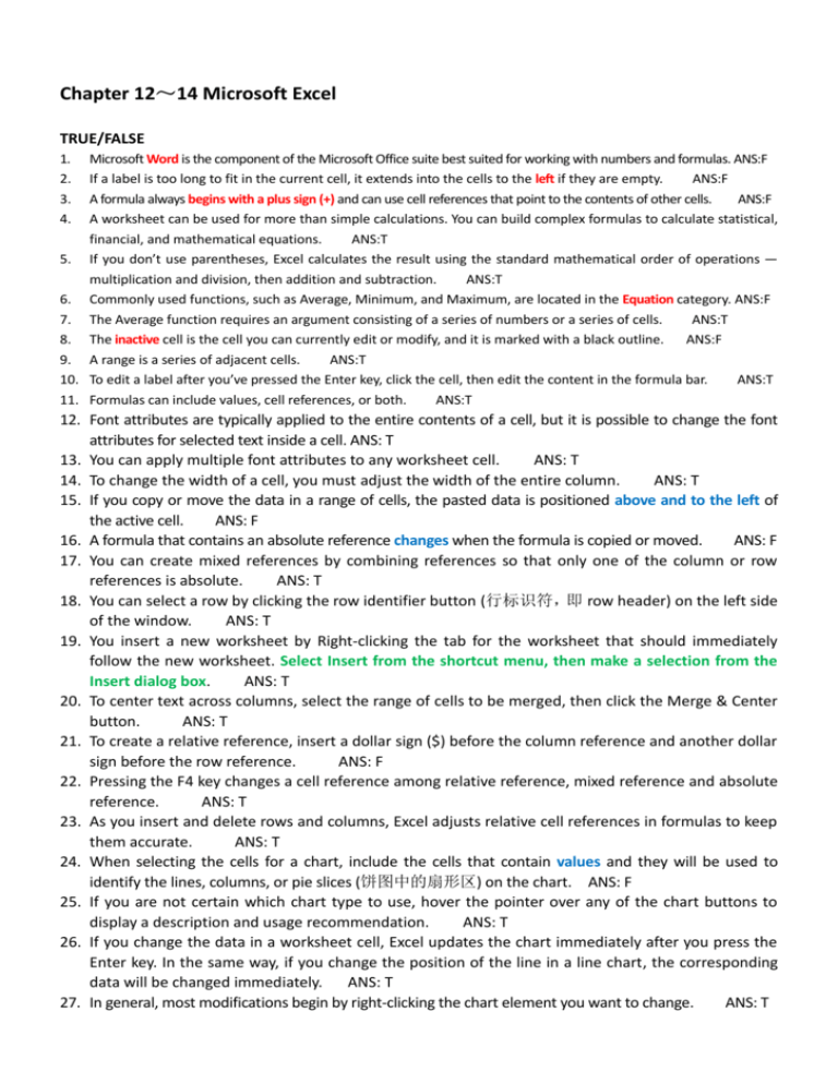
Chapter 12～14 Microsoft Excel
TRUE/FALSE
1.
2.
3.
4.
Microsoft Word is the component of the Microsoft Office suite best suited for working with numbers and formulas. ANS:F
If a label is too long to fit in the current cell, it extends into the cells to the left if they are empty.
ANS:F
A formula always begins with a plus sign (+) and can use cell references that point to the contents of other cells.
ANS:F
A worksheet can be used for more than simple calculations. You can build complex formulas to calculate statistical,
financial, and mathematical equations.
ANS:T
5. If you don’t use parentheses, Excel calculates the result using the standard mathematical order of operations —
multiplication and division, then addition and subtraction.
ANS:T
6. Commonly used functions, such as Average, Minimum, and Maximum, are located in the Equation category. ANS:F
7. The Average function requires an argument consisting of a series of numbers or a series of cells.
ANS:T
8. The inactive cell is the cell you can currently edit or modify, and it is marked with a black outline. ANS:F
9. A range is a series of adjacent cells.
ANS:T
10. To edit a label after you’ve pressed the Enter key, click the cell, then edit the content in the formula bar.
ANS:T
11. Formulas can include values, cell references, or both.
ANS:T
12. Font attributes are typically applied to the entire contents of a cell, but it is possible to change the font
attributes for selected text inside a cell. ANS: T
13. You can apply multiple font attributes to any worksheet cell.
ANS: T
14. To change the width of a cell, you must adjust the width of the entire column.
ANS: T
15. If you copy or move the data in a range of cells, the pasted data is positioned above and to the left of
the active cell.
ANS: F
16. A formula that contains an absolute reference changes when the formula is copied or moved.
ANS: F
17. You can create mixed references by combining references so that only one of the column or row
references is absolute.
ANS: T
18. You can select a row by clicking the row identifier button (行标识符，即 row header) on the left side
of the window.
ANS: T
19. You insert a new worksheet by Right-clicking the tab for the worksheet that should immediately
follow the new worksheet. Select Insert from the shortcut menu, then make a selection from the
Insert dialog box.
ANS: T
20. To center text across columns, select the range of cells to be merged, then click the Merge & Center
button.
ANS: T
21. To create a relative reference, insert a dollar sign ($) before the column reference and another dollar
sign before the row reference.
ANS: F
22. Pressing the F4 key changes a cell reference among relative reference, mixed reference and absolute
reference.
ANS: T
23. As you insert and delete rows and columns, Excel adjusts relative cell references in formulas to keep
them accurate.
ANS: T
24. When selecting the cells for a chart, include the cells that contain values and they will be used to
identify the lines, columns, or pie slices (饼图中的扇形区) on the chart. ANS: F
25. If you are not certain which chart type to use, hover the pointer over any of the chart buttons to
display a description and usage recommendation.
ANS: T
26. If you change the data in a worksheet cell, Excel updates the chart immediately after you press the
Enter key. In the same way, if you change the position of the line in a line chart, the corresponding
data will be changed immediately. ANS: T
27. In general, most modifications begin by right-clicking the chart element you want to change.
ANS: T
28. Excel can check the spelling of all labels in a worksheet and shows misspelled words with wavy red
underlines.
ANS: F
29. It’s a good idea to use the Save option to rename and save an extra copy of your worksheet before
testing, just in case your test significantly changes the worksheet.
ANS: F
COMPLETION
1.
2.
3.
4.
A(n) ________ consists of a grid of columns (214=16384, A～XFD) and rows(220=1048576).
ANS: worksheet
Excel worksheets are saved in a(n) ________.
ANS: workbook
In addition to writing your own formulas, you can use predefined formulas called ________.
ANS: functions
Excel includes many ________ functions such as average and normal distribution (正态分布). ANS: statistical
5. In addition to font attributes, you can also apply ________ formats—currency, percent, commas, and
decimals—to cells that contain values.
ANS: number
6. To quickly select all cells in a column, click the column ________ at the top of the column. ANS: header
7. Excel treats all cell references as ________ references unless you specify otherwise.
ANS: relative
8. To insert more than one row at a time, drag down over the number of rows you want to insert.
________ click the row headers then select Insert in the shortcut menu.
ANS: Right
9. The ________ function can be used to hide rows or columns you don’t want displayed. ANS: Hide
10. A(n) ________ chart is used to show data that changes over time.
ANS: line 折线图用于表现同
一数据序列的变化趋势
11. A(n) ________ chart illustrates the proportion of parts to a whole.
ANS: pie 饼状图用于表现数
据间的比例关系
12. A(n) ________ chart (sometimes called a column chart) is used to show comparisons.
ANS: bar
柱形图用于组间数据的比较
13. The round, green handle that appears at the top of a graphic allows you to ________ the graphic. ANS: rotate
14. Excel’s ________ view helps you refine(改善) the appearance of a worksheet before you print it or
post it as a Web page.
ANS: Page Layout
15. _____ orientation prints a worksheet on a vertically oriented page. ANS: Portrait(Landscape 为横版)
16. ________, the lines that separate one cell from another, can be printed to create visual boundaries
for rows and columns.
ANS: Gridlines
17. A(n) ________ is text that appears at the top of every page and a footer is text that appears at the
bottom of every page.
ANS: header
MULTIPLE CHOICE
1.
2.
3.
4.
5.
6.
7.
8.
A worksheet ____ is the rectangle formed by the intersection of a column and row.
A. entry
B. blank C. input D. cell
ANS:D
Table rows are typically labeled with ____. A. letters
B. numbers C. names D. formulas
ANS:B
A ____ contains one or more worksheets, each represented by a tab at the bottom of the Excel window.
A. workbook
B. journal C. theme D. workgroup
ANS:A
Values can be entered automatically using the fill handle and a technique called ____.
A. drag-and-drop
B. cut-and-paste C. copy-and-paste D. drag-and-fill
ANS: D
If you want to specifically enter a number as a label, you can type a(n) ____ before the number.
A. asterisk
B. apostrophe C. question mark D. equal sign
ANS:B
With the Auto Fill Options button, you can fill the selection with ____.
A. a series of numbers
B. the value of the initial cell with or without cell formatting
C. cell formatting
without a value D. any of the above
ANS: D
Operations within ____ are completed first.
A. brackets
B. parentheses C. quotation marks D. question marks ANS:B
If you don’t use parentheses, Excel calculates the result using the standard mathematical order of operations with ____ first.
9.
10.
11.
12.
13.
14.
15.
16.
17.
18.
19.
20.
A. multiplication and division B. addition C. subtraction D. formulas ANS: A
You can edit a formula after you’ve pressed the Enter key ____.
A. in the cell
B. in the formula bar C. either a. or b. D. neither a. nor b.
ANS:C
The easiest way to create a formula is to use the ____ method.
A. list
B. pointer C. copy D. type
ANS:B
A rectangle of dashes around the selected cell is called a ____.
A. marquee B. sign C. border
D. billboard ANS:A
The most common arithmetic ____ are - (subtraction), + (addition), * (multiplication), / (division), % (percent), and
^ (exponent).
A. formulas
B. integers C. calculators D. operators
ANS:D
A ____ specifies how to add, subtract, multiply, divide, or otherwise calculate the values in worksheet cells.
A. formula
B. cell reference C. cell D. label
ANS:A
A ____ is the column and row location of a cell.
a. formula
B. cell reference C. value D. label
ANS:B
A ____ is any text entered into a cell of the worksheet. a. formula B. cell reference c. label d. value ANS:C
You can use ____ for a worksheet title, to describe the numbers you’ve entered in other cells, and for text data,
such as the names of people or cities.
a. values
B. labels C. formulas D. cell references
ANS:B
Any numerical data you do not intend to use in a calculation should be entered as a ____.
A. format
B. label C. value D. cell reference
ANS:B
A(n) ____ is a formula that references the cell in which the formula resides.
A. cell reference B. circular reference
C. backwards reference D. infinite reference ANS:B
Excel includes more than ____ functions from which you can choose. a. 100
B. 250 C. 400 D. 550
ANS:B
You can use the ____ button to select a function from a list.
A. Insert Formula
B. Insert Function
C. Improve Formula
D. Improve Function
ANS:B
21. You can use the ____ function to calculate all types of loan payments, such as those for a car or for a house.
A. PMT
B. COUNT C. AVERAGE D. SUM
ANS:A
22. To select a range of cells for use as arguments in a function, click the ____ that contains data you want to use in
the function, then drag down to the bottom-right cell.
A. upper-left cell
B. upper-left row label C. upper-left column label D. none of the above
ANS:A
23. If a label is too long to fit in the current cell, it extends into the cells ____ if they are empty.
A. to the right
B. to the left C. directly above D. directly below
ANS: A
24. When you complete the Average function, the result is calculated as an average of the values in the ____. ANS: A
A. cells you specified B. column containing the active cell C. row containing the active cell D. entire worksheet
25. Use the ____ button to quickly create a function to calculate the total of a column or row of cells.
A. AutoSum C. AutoFunction
B. AutoCalculate D. AutoFormula
ANS: A
26. AutoSum works best if every cell in the row or column of cells contains a ____.
A. label
B. value C. either a. or b. D. neither a. nor b.
ANS:B
27. If the AutoSum button does not automatically select the correct cells, press the ____ key to remove the function
and create the Sum function manually.
A. Delete
B. Esc C. Backspace D. End
ANS:B
28. Commonly used functions, such as Sum, Average, Minimum, and Maximum, are located in the ____ category.
A. Calculation C. Operator
B. Formula D. Statistical
ANS: D
29. A(n) ____ consists of values or cell references used to calculate the result of the function.
A. formula
B. reference C. argument D. parameter
ANS: C
30. Excel includes many ________ functions such as payments and net present value (净现值), and mathematical and
trigonometric functions (三角函数) such as absolute value and arctangent(反正切).
A. financial
B. statistical
C. mathematical D. date and time ANS: A
31. The ____ button puts a border around the outside edges of selected cells.
A. Outline
B. Border
C. Shading
D. Selection
ANS: A
32. The ____ button adds borders between individual cells.
A. External
B. Internal
C. Outside
D. Inside
ANS: D
33. The Percent Style button displays cell contents as a percentage, which means .35 is displayed as ____.
A. .35%
B. 3.5%
C. 35%
D. 350%
ANS: C
34. By default, labels are aligned on the ____ of a cell.
A. right edge
B. left edge
C. center
D. none of the above
ANS: B
35. Typically, you’ll want to ____ the headings for columns of numbers.
A. center
B. right-align
C. either a. or b.
D. neither a. nor b.
ANS:C
36. A cell reference that changes when a formula is copied or moved is called a(n) ____ reference.
A. absolute
B. relative
C. formula
D. mixed
ANS: B
37. As with Microsoft Word, Excel allows you to work with either predefined or custom ____.
A. labels
B. styles C. themes D. values ANS: B
38. ____ styles are built into the software, and include formats for displaying currency, percentages, and
general numbers.
A. Template
B. Predefined
C. Smart
D. Custom
ANS: B
39. To hide a block of rows or columns, first select the rows or columns to be hidden, ____ the
highlighted area, then select Hide.
A. left-click
B. right-click
C. double-click the left mouse button
D. double-click the right
mouse button
ANS: B
40. To display rows or columns that were previously hidden, select the rows or columns that border the
hidden section. Right-click, then choose ____.
A. Reveal
B. Unhide
C. Display
D. Show
ANS: B
41. A workbook—sometimes called a “3D workbook”—is a collection of ____.
A. spreadsheets
B. tables
C. formulas
D. worksheets
ANS: D
42. The default workbook contains three worksheets, titled ____.
A. Sheet1, Sheet2, and Sheet3
C. WB1, WB2, and WB3
B. WS1, WS2, and WS3
D. File1,
File2, and File3
ANS: A
43. Click the tabs ____ of the screen to navigate through the worksheets.
A. at the top
B. at the bottom
C. on the right-side
D. on the left-side
ANS: B
44. You can ____ by right-clicking a worksheet tab and making a selection from the shortcut menu.
A. rename worksheets
B. change the color of the tabs
C. change the order of the
worksheets
D. all of the above
ANS: D
45. If you need to perform a multilevel sort, add additional levels with the Add Level button and
designate(指定) the columns from the ____ list.
A. Add columns
B. Add new
C. Then sort
D. Then by
ANS: D
46. If the chart doesn’t seem to make sense(让人看不明白——此处指横纵坐标系搞反了), make sure
the chart is selected and try clicking the Switch Row/Column button in the ____ group on Design
subTab within ChartTools contextsual Tab.
A. Page
B. Data
C. Chart
D. Format
ANS: B
47. By default, the chart is inserted into the current worksheet. You can move the chart with the Move
Chart button on the ____ tab.
A. Home
B. Edit
C. Design
D. Format
ANS: C
48. To select a different chart type, select the Design tab, and then click the ____ button.
A. Change Chart Type B. Swap Chart Type C. Format Chart Type D. Choose Chart Type ANS: A
49. When making changes to a chart, make sure the chart is selected so that Excel displays all of the
charting tabs which includes ____.
A. Design
B. Layout
C. Format
D. all of the above
ANS: D
50. To select a different range of cells to be charted, click the ____ button from the Design tab.
A. Choose Data
B. Data Range
C. Data Design
D. Select Data
ANS: D
51. Graphics can be resized using the ____ “handles” that appear on the edges of a selected graphic.
A. round
B. triangular
C. square
D. rectangle
ANS: A
52. In the Clip Art task pane, enter a ____, such as animal, for the type of clip art you would like to use
in the Search for text box, then click Go. Choose an image from the available pictures, and then close
the Clip Art task pane.
A. keyword
B. filename
C. definition
D. address
ANS: A
53. You can select a specific area of a worksheet to print. When you use the Print ____ button in
PageSetup group on Page Layout tab to select such an area, the setting is used every time you print.
A. Preview
B. Area
C. Range
D. Setting
ANS: B
54. If you want headings displayed and printed, make sure there are checkmarks in the Headings ____
and Print boxes.
A. Show
B. View
C. Display
D. On
ANS: B
55. In Page Layout view, gridlines are shown in light ____ unless you turn them off.
A. red
B. yellow
C. green
D. gray
ANS: D
56. To enter Page Layout view, click the ____ tab, then select Page Layout.
A. Cells
B. Numbers
C. View
D. Print
ANS: C
57. Excel provides several ways to access margin settings, but one of the easiest ways is to drag directly
in the margins while in ____ view.
A. Page Layout
B. Page Setup
C. Print Dialog
D. Print area
ANS: A
58. If your worksheet contains multiple pages, the margin settings apply to ____.
A. selected pages B. all pages C. the page you are currently viewing D. the first page
ANS: B
59. A ____ is text that appears at the bottom of every page.
A. header
B. footer
C. footnote
D. note
ANS: B
60. If you would like to specify header on the left side of even numbered pages, but on the right side of
odd numbered pages there are no header content, you would choose the following header and
footer option: ____.
A. Different First Page
B. Different Odd and Even Pages
C. Scale with Document
D. Align
with Page Margins
ANS: B
61. To specify the order in which pages of a multipage worksheet are printed, use the ____ tab of the
Page Setup dialog box. A. Workbook
B. Sheet
C. File
D. Order
ANS: B
62. You might want to insert a ____ page break if a page ends with a row that should be grouped with
data on the next page.
A. manual
B. automatic
C. style
D. format
ANS: A
63. To print only the current worksheet, select the Print ____ option instead of the Print Entire
Workbook option.
A. Active sheet(s)
B. Current sheet(s)
C. Entire sheet(s)
D. Chosen sheet(s)
ANS: A
64. Before you save a worksheet as a Web page, it’s a good idea to save it in normal Excel ____ format.
A. .xlsx
B. .ws
C. .wks
D. .wbk
ANS: A
65. The active cell can be identified in all of the following ways except ____.
ANS: A
A. a block arrow displays in the center of the cell B. the active cell reference displays in the Name box
C. a heavy border surrounds the cell
D. the column heading and row heading are highlighted
66. The ____ is the small black square located in the lower-right corner of the heavy border around the
active cell (or range).
A. sizing handle B. fill handle C. move handle D. marquee
ANS: B
67. When one range is copied to another, Excel displays the ____ that can be used to choose whether to
copy the value with formatting, without formatting, or only copy the format. ANS: C
A. Auto Sum Options button
B. AutoCorrect Options button
68.
69.
70.
71.
72.
C. Paste Options button (or: Auto Fill Options button)
D. AutoComplete Options button
The small box to the right of an embedded column chart contains the legend, which ____. ANS: B
A. supplies the title of the chart
B. identifies each bar in the chart
C. determines the increments along the y-axis
D. all of the above
When the Tools button in the Save As dialog box is clicked, the ____ in the list that displays allows a
backup copy of the workbook to be saved, a password to limit access to the workbook to be created,
and other functions to be carried out. ANS: D
A. Add to Favorites command
B. Web Options command
C. Properties command
D. General Options command
Right click the status bar, you may customize it with the short cut menu. Which of the following
items may be shown in status bar? ANS: D
A. Sum
B. Average C. Maximum D. All of the above
Double-clicking in a cell, Excel switches to ____, the active cell contents display in the formula bar,
and a flashing insertion point displays in the active cell. ANS: B
A. Replace mode
B. Edit Mode (Enter mode)
C. Overtype mode
D. Ready mode
Excel provides the Undo command on the ____ that can be used to erase the most recent
worksheet entries. ANS: A
A. Quick Access Toolbar
B. Insert Tab
C. Home Tab
D. View Tab
73. To start a new line in a cell, press ____ after each line, except for the last line, which is completed by pressing
the ENTER key, or pressing one of the arrow keys. ANS: A
A. ALT+ENTER
B. ICTRL+ENTER
C. SHIFT+ENTER
D. TAB+ENTER
74. The ____ preceding a formula is an important part of the formula: it alerts Excel that a formula or function is
being entered and not text. ANS: D
A. number sign (#)
B. dollar sign ($)
C. percent sign (%)
D. equal sign (=)
75. To select the nonadjacent range B5, C10, and D10, select cell B5, and then, while holding down the ____ key,
drag through the range C10:D10. ANS: C
A. SHIFT
B. ALT
C. CTRL
D. HOME
76. To display a hidden column, position the mouse pointer to the ____. ANS: D
A. left of the column heading boundary where the hidden column is located and then drag to the right
77.
78.
79.
80.
B. right of the column heading boundary where the hidden column is located and then drag to the left
C. left of the column heading boundary where the hidden column is located and then drag to the left
D. right of the column heading boundary where the hidden column is located and then drag to the right
If the adjacent two cells containing 780 and 760 are copied using the fill handle, the next three values of the
extended series will be ____. ANS: B
A. 780, 760, 780
B. 740, 720, 700
C. 680, 660, 580
D. 775, 770, 765
If a cell containing 10 is copied using the fill handle, the next three values of the extended series will be ____. ANS: C
A. 11, 12, 13
B. 9, 8, 7
C. 10, 10, 10
D. 20, 20, 40
If a cell containing 10 is copied using the fill handle holding down the CTRL key, the next three values of the
extended series will be ____. ANS: A
A. 11, 12, 13
B. 9, 8, 7
C. 10, 10, 10
D. 20, 20, 40
If a cell containing the date 11-26-2014 is copied using the fill handle, the next three values of the extended series will be
____. ANS: D
A. 11-25-2014, 11-24-2014, 11-23-2014
B. 11-26-2014, 11-26-2014, 11-26-2014
C. 12-26-2014, 1-26-2015, 2-26-2015
D. 11-27-2014, 11-28-2014, 11-29-2014
81. If a cell containing the date 11-26-2014 is copied using the fill handle holding down the CTRL key, the next
three values of the extended series will be ____. ANS: B
A. 11-25-2014, 11-24-2014, 11-23-2014
B. 11-26-2014, 11-26-2014, 11-26-2014
C. 12-26-2014, 1-26-2015, 2-26-2015
D. 11-27-2014, 11-28-2014, 11-29-2014
82. If a cell containing July is copied using the fill handle, the next three values of the extended series will be ____.
ANS: C
A. July, July, July
B. June, May, April
C. August, September, October
D. 8, 9, 10
83. To input 10 in all of the cells within a range, select the range and type 10 then press ENTER holding down the ____
key. ANS: B
A. SHIFT B. CTRL C. ALT D. TAB
84. If the result a formula should produce is known(如
果
某
个
公
式
的
结
果
是
已
知
的
), the ____ command in data tab can be used to
determine the value of a cell on which the formula depends. ANS: D
A. Track Changes
B. Data Analysis
C. Share Workbook
D. Goal Seek
85. Goal seeking assumes the value of ____ referenced directly or indirectly can be changed. ANS: B
A. no cells
B. only one cell
C. two or more cells
D. any number of cells
86. The mouse pointer turns to a ____ whenever you move it outside the worksheet. ANS: B
A. hand
B. left (hand) point arrow
C. double-headed arrow
D. crosshair
87. The ______ key selects the leftmost cell of the current row. ANS: C
A. Page Down
B. End
C. Home
D. Insert
88. The basic unit of a worksheet into which you enter data is called a ____ . ANS: B
A. tab B. cell C. box D. range
89. The vertical axis(垂直轴) of a chart is called the ____ axis. ANS: C
A. long
B. range
C. value
D. floating
90. To enter a number as text, start the entry with a(n) ____ . It means number stored as text.
B. hyphen
A. asterisk
C. semicolon
ANS: D
D. apostrophe (英文的单撇)
91. The horizontal and vertical lines on a worksheet are called ____, they form the cells.
A. cells
B. sheets
C. blocklines
D. gridlines (栅格线、网格线)
92. The area on a worksheet where the chart appears is called the ____. ANS: D
A. x-axis
B. chart bed
C. chart cell
D. chart location
ANS: D
93. Holding down the ____ key while dragging a chart’s sizing handles snaps (aligns) the new border to the
worksheet gridlines.
A. Alt
B. CTRL
ANS: A
C. Shift
D. Ctrl+Shift
94. A column letter above the grid, also called a ____, identifies each column.
ANS: A
A. column heading (列标题)
B. column reference
C. row heading
D. table reference
95. The ______ function counts the number of cells in a range that contain numbers.
ANS: C
A. TOTAL
B. NUMBER
C. COUNT 数指定区域中包含数值的单元格个数
D. MIN
96. Excel’s ____ provides a convenient way to add the numbers in cells.
ANS: B
A. AVERAGE function
B. SUM function
C. COUNT function
D. INT function
97. The ____ function sums the numbers in a specified range and then divides the sum by the number of non-zero
ANS: B
B. AVERAGE
C. MAX
cells in the range.
A. MIN
D. COUNT
ANS: D
B. IF(logical_test, value_if_false, value_if_true)
C.IF(value_if_false, logical_test, value_if_true)
D. IF(logical_test, value_if_true, value_if_false)
98. The general form of the IF function is ____ .
A. IF(value_if_true, logical_test, value_if_false)
99. The IF function =IF(B4>=$B$22,B4, $B$22) is assigned to cell B8. If the value in cell B4 is 66, the value in cell
B22 is 65, Excel displays ____ in cell B8.
ANS: A
A. 66
B. 1
C. 65
D. -1
100. You can display tomorrow's date in a cell by using ______.
B. TODAY() + 1
A. NOW()
C. TODAY()
ANS: B
D. TOMORROW
101. To apply a Percent style format to a cell using shortcut keys, press ____ .
A. ALT+PERCENT SIGN
C.CTRL+PERCENT SIGN
ANS: D
B. ALT+SHIFT+PERCENT SIGN
D. CTRL+SHIFT+PERCENT SIGN
ANS: C
102. To select a range of cells using the keyboard, holding ____ then use the arrow keys.
A. Ctrl
B. Alt
C.Shift
D.Tab
103. Every time you enter a value into a cell in the worksheet, Excel ____ all formulas.
ANS: A
A. recalculates
B. cancels
C. highlights
D. displays
104. The ____ button on the Home Tab allows you to format a cell quickly by copying a cell’s format to another cell.
ANS: B
A. Merge and Center
B. Format Painter
C. Drawing
D. Format Cell
ANS: C
105. With a 3-D pie chart, you can explode ____ of the slices.
A. 1
B. as many as 2
C. all
D. none
ANS: A
C.separated pie chart D. highlighted pie chart
106. A pie chart with one or more slices offset from the main portion is called a(n) ____.
A. exploded pie chart 分离型饼图 B.detached pie chart
107. To select nonadjacent ranges, select the first range, hold down the ______ key, and then select the next range.
ANS: C
A. SHIFT
B. ALT
C. CTRL
D. HOME
108. To select a range, select the first cell, hold down the _____ key, and then select another cell on the diagonal corner.
ANS: A
A. SHIFT
B. ALT
C. CTRL
D. HOME
109. When working with a large worksheet, you can split the window into two or four window ____ to view different
parts of the worksheet at the same time.
B. panes
A. segments
ANS: B
C. sections
D. views
110. The bar going across the middle of the window is called the ____ .
ANS: D
A. horizontal ruler
B. scroll bar
C. vertical split bar
D. horizontal split bar
111. If you freeze the titles in your worksheet, they will remain frozen until you click the ____ command in Window group on
ANS: C
View Tab.
B. Split
A. Freeze Panes
C. Unfreeze Panes
D. Titles
112. To toggle between formula view and value view of a worksheet, press ____ key.
A. CTRL + ”
B. CTRL + ` (Tab 上方的那个 ACCENT 键，和英文的单撇反方向)
ANS: B
C. CTRL + ^
D. CTRL + !
113. By default, the original data (formula, function) inputted in a cell is displayed in the _____, the cell shows the
value.
ANS: B
A. Name box
B. formula bar
C. Insert Function box
D. status bar
114. To specify an absolute reference in a formula, enter a(n) ___ before a column letter and a row number.
ANS:
C
A. percent sign
B. apostrophe
C. dollar sign
D. tilde
115. To switch between relative reference and absolute reference in a formula, put the intersection in the formula bar
then press ____ key.
A. F1
B. Shift
ANS: D
C. Ctrl
D. F4
116. Which one of the following formulas includes absolute reference?
A. = $A$2+$B$2
B. = $A2+$B2
C. = A2+B2
117. Which one of the following formulas includes relative reference?
A. = $A$2+$B$2
B. = $A2+$B2
C. = A2+B2
ANS: A
D. = A$2+B$2
ANS: C
D. = A$2+B$2
118. Which one of the following formulas includes mixed reference (relative column and absolute row)?
A. = $A$2+$B$2
B. = $A2+$B2
C. = A2+B2
D. = A$2+B$2
ANS: D
ANS: B
119. Which one of the following formulas includes mixed reference (absolute column and relative row)?
A. = $A$2+$B$2
B. = $A2+$B2
C. = A2+B2
D. = A$2+B$2
120. Excel displays the error message ____ in cells to indicate a cell reference error.
ANS: D
A. #VALUE!
B. #DIV/0!
C. #NAME?
D. #REF!
121. Excel displays the error message _____ in cells to indicate unknown cell name occurs in the formula or function.
ANS: C
A. #VALUE!
B. #DIV/0!
C. #NAME?
D. #REF!
122. Excel displays the error message _____ in cells to indicate the denominator (分母) is zero now.
ANS: B
A. #VALUE!
B. #DIV/0!
C. #NAME?
D. #REF!
123. Excel displays the error message ____ in cells to indicate the value of the cell you referenced can’t be calculated.
A. #VALUE!
B. #DIV/0!
C. #NAME?
D. #REF!
ANS: A
124. Excel displays the message ____ in cells to indicate the width of the column isn’t wide enough.
A. ####
B. ****
C. ????
ANS: A
D. !!!!
125.
To manually adjust the width of a column, position the pointer over the vertical line between
the two column headings of the current column and the right side column, so that the pointer
changes to a shape. ____ while you drag the vertical line left or right to manually adjust the width of
the column.
ANS: D
A. Double-click the right mouse button
B. Double-click the left mouse button
C. Press and
hold the right mouse button
D. Press and hold the left mouse button
126. The worksheet entries that determine the high of the columns in a chart are called the ____ .
ANS: A
A. data series
B. pie data
C. data collection
D. chart data
127. The entries that will identify the clusters (簇) of columns in a chart are called ____ .
ANS: A
A. category names
B. values
C. slice names
D. none of the above
128. A ____ shows the system date of which your computer keeps track.
ANS: A
A. date stamp
B. system stamp
C. date marker
D. date formatter
129. You can apply ____ that appears only when the value in a cell meets conditions that you specify.
ANS: D
A.specified formatting B.narrow formatting C.customized formatting D.conditional formatting
130. When you name a cell, if the name is made up of two or more words, you replace any space with a(n) ______.
ANS: A
A. underscore character ( _ )
B. asterisk ( * )
C. ampersand ( & )
131. Cells that you cannot change values in are called ______.
D. pound ( # )
ANS: A
A. protected cells
B. unprotected cells
C. saved cells
D. guarded cells
132. To bold the font of the entire worksheet, press CTRL+A or click the ______ button immediately above row
heading 1 and left column heading A, then click the Bold button on the Formatting toolbar
ANS: D
A. Worksheet
B. Select Worksheet
C. Apply To All
D. Select All
133. To name a cell or a range of cells (or remove a defined name), click ______ in Defined Names group on
Formulas tab then click New button (or select the defined name click Delete button). Or you input a meaning
name in the Name Box directly then press ENTER.
ANS: D
A. Tools
B. Edit
C. File
D. Name Manager
134. Hiding is a technique you can use to hide data that might be sensitive or not relevant to a report. Which of the
following can be hided in Excel?
A. rows and columns
ANS: D
B. worksheets
C. workbook
D. All of the above
ANS: D
C. tilde (~)
D. ampersand ( & )
135. The ______ is the concatenation operator (连接符).
A. asterisk (*)
B. percent sign (%)
136. To get the summation of the union (并集) of the two ranges A2:A3 and B4:C4, you select the function SUM().
Which one of the following operator should be put between the two ranges?
A. asterisk (*)
B. space ( )
C. comma (,)
D. colon (:)
ANS: C
137. To get the summation of the intersection (交集) of the two ranges A1:B4 and A3:D4, you select the function
SUM(). Which one of the following operator should be put between the two ranges?
A. asterisk (*)
B. space ( )
C. comma (,)
138. Data is in ______ if it is sorted from Z to A.
ANS: B
D. colon (:)
ANS: B
A. alphabetical order
B. descending order(降序)
C. ascending order(升序)
D. downward order
139. If you need to sort by more than one criterion, you should use the Sort Dialog Box. Click Sort command in Sort
& Filter group on ____ tab.
A. Insert
B. Data
ANS: B
C. Home
D. View
140. Excel is not ______, meaning it considers uppercase and lowercase characters in a comparison criterion (比较
标准) to be the same.
ANS: C
A. case-definite
B. case-exact
C. case-sensitive 大小写敏感
D. case-final
141. The ______ option on the Paste menu will paste the formulas and formats from the source area, but switch the
columns and rows.
ANS: D
A. Formulas
B. Paste Special
C. Switch
D. Transpose (转置)
142. If the cell referenced by a formula locates in a different worksheet, which one of the following character should
be followed the worksheet’s name?
A. #
B. !
C. *
ANS: B
D. [ ]
143. If the cell referenced by a formula locates in a different workbook, which one of the following character should
be put on both side of the workbook’s name?
A. #
B. !
C. *
ANS: D
D. [ ]
144. A range that spans two or more worksheets in a workbook is called a ______.
A. double range
B. 3-D range
C. extended range
ANS: B
D. multiple range