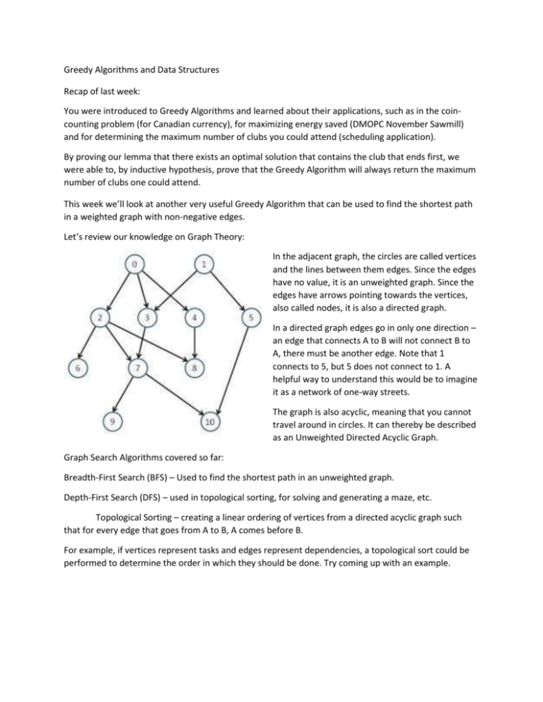
Greedy Algorithms and Data Structures
Recap of last week:
You were introduced to Greedy Algorithms and learned about their applications, such as in the coincounting problem (for Canadian currency), for maximizing energy saved (DMOPC November Sawmill)
and for determining the maximum number of clubs you could attend (scheduling application).
By proving our lemma that there exists an optimal solution that contains the club that ends first, we
were able to, by inductive hypothesis, prove that the Greedy Algorithm will always return the maximum
number of clubs one could attend.
This week we’ll look at another very useful Greedy Algorithm that can be used to find the shortest path
in a weighted graph with non-negative edges.
Let’s review our knowledge on Graph Theory:
In the adjacent graph, the circles are called vertices
and the lines between them edges. Since the edges
have no value, it is an unweighted graph. Since the
edges have arrows pointing towards the vertices,
also called nodes, it is also a directed graph.
In a directed graph edges go in only one direction –
an edge that connects A to B will not connect B to
A, there must be another edge. Note that 1
connects to 5, but 5 does not connect to 1. A
helpful way to understand this would be to imagine
it as a network of one-way streets.
The graph is also acyclic, meaning that you cannot
travel around in circles. It can thereby be described
as an Unweighted Directed Acyclic Graph.
Graph Search Algorithms covered so far:
Breadth-First Search (BFS) – Used to find the shortest path in an unweighted graph.
Depth-First Search (DFS) – used in topological sorting, for solving and generating a maze, etc.
Topological Sorting – creating a linear ordering of vertices from a directed acyclic graph such
that for every edge that goes from A to B, A comes before B.
For example, if vertices represent tasks and edges represent dependencies, a topological sort could be
performed to determine the order in which they should be done. Try coming up with an example.
Review of BFS:
Running BFS on a weighted directed graph where the
vertices represent cities and the edges represent the cost
of a train ticket to find the cheapest path from A to F:
It would tell us that the lowest cost of getting from A to F
is 12. Why is this not correct?
Is there another algorithm we could come up with?
Dijkstra’s Algorithm:
Each node will have a distance value from A. If it is unexplored, that value is set to infinity,
Start at A, add vertices adjacent to A into Explore list. Mark A as visited.
Visited: A (0) - The value in parentheses is the lowest cost of travelling from A to that point.
Explore: B (1) - The value in parentheses is the cost of visiting B from A.
-
Greedy Part: Choose the city that is the cheapest to get to
Visit B, add vertices adjacent to it to the Explore list.
Visited: A (0), B (1)
Explore: C (4), E (12), D (3) - The value for each node is the distance from A. Until it is visited, that value
may be replaced with a lower one.
Visit D, add vertices adjacent to it to the Explore list.
Visited: A (0), B (1), D (3)
Explore: C (4), E (5) Notice that G is not adjacent to D and that E’s value was updated with a lower one.
Visit C as it is the cheapest to get to. It is also adjacent to E, but the cost of getting there via C is 8.
Visited: A (0), B (1), C (4), D (3)
Explore: E (5)
Visit E and add F to the Explore queue.
Visited: A (0), B (1), C (4), D (3), E (5)
Explore: F (8)
We visit F, our destination, and output 8 as the cost of the cheapest route.
Visited: A (0), B (1), C (4), D (3), E (5), F (8)
Running Time Analysis: O(V2), where V is the number of vertices. In the worst case, we would visit every
node O(V) and when choosing the next node to visit after visiting one, we would select the closest one,
which would take O(V). Multiplying the two, we obtain a worst-case running-time of O(V2).
Can we do better? Of course!
The bottleneck is in choosing which city to explore next: Our goal is to quickly find the minimum from
the Explore list. As of now, it takes O(n), where n is the number of vertices in the list.
-
Binary Search: takes lg(n) to find insertion point, but O(n) to add into list as to keep it sorted.
Binary Heap:
Advantages:
-
Can obtain maximum or minimum in O(1) – yes, you read that right, constant time!
Takes O(lg n) to insert a value or to remove the head of the heap.
How it works:
Insert-min: Add element to a leaf node, keep
shifting upwards until it conforms to the heap
property. O(lg n)
Find-min: Simply get the head of the heap.
O(1)
Delete-min: Swap the head with a leaf node.
Delete the head and keep swapping the new
head node downwards until it conforms to the
heap property. O(lg n)
Implementation: Can be implemented using a simple array:
Let n be the number of elements in the heap and i be an index of the array storing the heap. If the tree’s
root is at index 0, with valid indices 0 through n − 1, then each element a at index i has children at
indices 2i + 1 and 2i + 2 and its parent floor((i − 1) ∕ 2).
But don’t worry, you won’t actually have to implement it. A heap is represented in Java by a
PriorityQueue, where you can add elements, remove the minimum, and specify how to compare the
elements through the use of a Comparator.
In Python, you can import heapq. Refer to the Python and Java documentation for examples.
A Proof of Correctness for Dijkstra’s Algorithm can be found here:
http://www.ieor.berkeley.edu/~ieor266/Lecture11.pdf