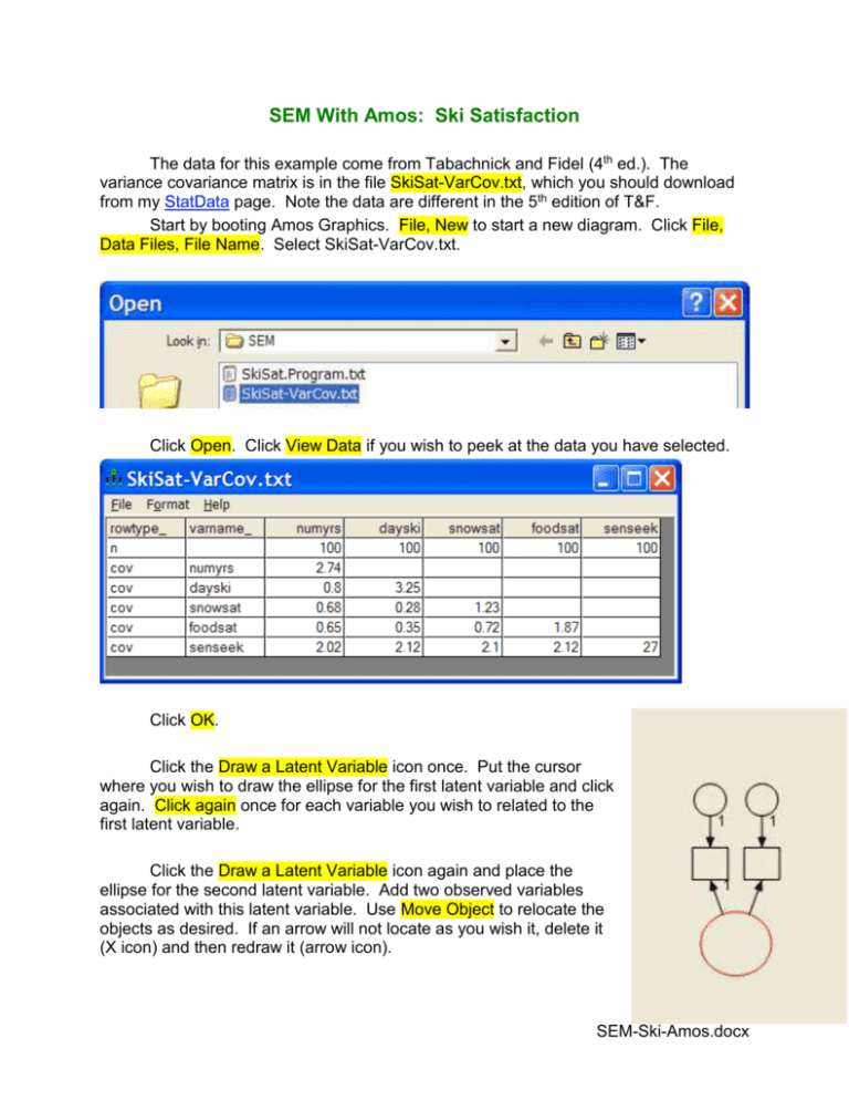
SEM With Amos: Ski Satisfaction
The data for this example come from Tabachnick and Fidel (4th ed.). The
variance covariance matrix is in the file SkiSat-VarCov.txt, which you should download
from my StatData page. Note the data are different in the 5th edition of T&F.
Start by booting Amos Graphics. File, New to start a new diagram. Click File,
Data Files, File Name. Select SkiSat-VarCov.txt.
Click Open. Click View Data if you wish to peek at the data you have selected.
Click OK.
Click the Draw a Latent Variable icon once. Put the cursor
where you wish to draw the ellipse for the first latent variable and click
again. Click again once for each variable you wish to related to the
first latent variable.
Click the Draw a Latent Variable icon again and place the
ellipse for the second latent variable. Add two observed variables
associated with this latent variable. Use Move Object to relocate the
objects as desired. If an arrow will not locate as you wish it, delete it
(X icon) and then redraw it (arrow icon).
SEM-Ski-Amos.docx
2
Click “File, Save As” and save your model before too
much time passes – that way, if AMOS decides to nuke your
model then you can get it back from the saved amw file. I try to
remember to save my model frequently while I am working on
it.
Click the Draw Observed Variables icon and locate an
observed variable near the second (right) latent variable. Place
an arrow going from it to the second latent variable.
Click the List Variables in Data Set icon and then drag
each variable name to the appropriate rectangle. You will find
that the rectangles are not large enough to hold the variable
names. Use the Change the Shape of Objects tool to enlarge
the rectangles.
Right click the error circle that goes to “numyrs.” Select Object Properties. Enter
“e1” as the variable name. In the same way name the other three error circles.
Use Object Properties to name the first latent variable (that on the left) “LoveSki.”
Click the Parameters tab and set the variance to 1. Name the second latent variable
“SkiSat,” but do not fix its variance. Draw an arrow from LoveSki to SkiSat.
3
Click the “Add a Unique Variable to an Existing Variable icon and then click the
SkiSat ellipse. Move and resize the error circle and name it “d2.”
Compare your diagram with that in Tabachnick and Fidell. Notice that AMOS
has fixed the coefficient from LoveSki to numyears at 1. That is not necessary, as we
fixed the variance of LoveSki to 1. Right click that arrow and select Object Properties.
Delete the “1” under Regression Weight.
4
Click the Analysis Properties icon. Under the Output tab select the stats you
want, as indicated below.
To start the analysis, just click the Calculate Estimates icon.
Click “Proceed with the analysis.”
5
Click the “View the output path diagram” to see the path diagram with values of
the estimated parameters placed on the arrows. Notice that you can select
unstandardized or standardized estimates.
The standardized regression coefficients are printed beside each path. Beside
each dependent variable is printed the r2 relating that variable to a latent variable(s).
Click the View Text icon to see much more extensive output from the analysis.
Under “Notes for model: Result” you see that the null that the model does fit the data
well is not rejected, 2(4) = 8.814, p = .066.
Under “Estimates” you see both unstandardized and standardized regression
weights. Many of the elements of the output are hyperlinks. For example, if you click
on the .399 estimate for the standardized regression weight for SkiSat <--- senseek, you
get the message “When senseek goes up by one standard deviation SkiSat goes up by
.399 standard deviation.”
The p values in the regression weights table are for tests of the null that the
regression coefficient is zero. Those in the variances tables are for tests of the null that
the variance is zero.
6
In the squared multiple correlations table the .328 for SkiSat indicates that 32.8%
of the variance in that latent variable is explained by its predictors (LoveSki and
SenSeek).
Look at the standardized residual covariances table. The elements in this table
represent differences between the sample variance/covariance table and the estimated
population variance/covariance table. The residuals for two covariances are
distressingly large – SenSeek-numyears and SenSeek-DaySki. We might want to
modify the model to reduce these residuals.
Total, direct, and indirect effects have the same meaning they had in path
analysis. For example, consider the standardized direct effect of LoveSki on FoodSat –
it is zero, as there is no path connecting those two variables. The indirect standardized
effect of LoveSki on FoodSat is the product of the standardized path coefficients leading
from LoveSki to FoodSat – that is, .411(.601) = .247. Of course, the total effects equal
the sum of the direct and indirect effects.
Under Modification Indices we see that the LM test indicates that allowing
LoveSki and SenSeek to covary would reduce the goodness of fit Chi-square by about
5.57. Since this involves only one parameter, this Chi-square could be evaluated on
one degree of freedom. It is significant. That is, adding this one parameter to the
model should significantly increase the fit of the model to the data.
Under Model Fit you see values of the many fit statistics. The Comparative Fit
Index (CFI) is supposed to be good with small samples, and we certainly have a small
sample here. Its value is .919. Values greater than .95 indicate good fit. The Root
Mean Square Error of Approximation (RMSEA) is .110. Values less than .06 indicate
good fit, and values greater than .10 indicate poor fit.
Modification of the Model
Our model does not fit the data very well.
Let us try adding the parameter recommended by the LM,
the path from SenSeek to LoveSki. Edit the diagram to look
like that below. Notice that LoveSki is now a latent dependent
variable. Also notice the following changes:
 LoveSki no longer has its variance fixed to 1 – AMOS
warned me not to constrain its variance to 1 if I wanted to
draw a path to it from SenSeek. Accordingly, I fixed the
regression coefficient from LoveSki to NumYrs at 1, giving
LoveSki the same variance as NumYrs. I had noticed earlier that LoveSki and
NumYrs were very well correlated.
 I added a disturbance for LoveSki, as it is now a latent dependent variable.
After making the indicated changes in the model, click the Calculate Estimates
icon and then view the output path diagram with standardized estimates.
7
e1
e3
1
1
numyrs
d1
snowsat
d2
1
1
1
LoveSki
1
SkiSat
dayski
foodsat
1
1
senseek
e2
e4
8
Click the View Text icon and look at the results. The goodness of fit Chi-square
is now only 2.053 on 3 degrees of freedom. Previously it was 8.814 on 4 degrees of
freedom. The change of fit Chi-square is 8.814  2.053 = 6.761 on (4  3) = 1 degrees
of freedom. Adding the path from SenSeek to LoveSki significantly increased the fit of
the model with the data.
Notice that the standardized residual matrix no longer has any very large
elements. Among the fit indices, the CFI has increased from .919 to 1.000 and the
RMSEA has decreased from .110 to 0.000, both indicating better fit.

Return to Wuensch’s Stats Lessons Page

An Introduction to Structural Equation Modeling (SEM)

SEM with SAS Proc Calis

Structural Equation Modeling using AMOS: An Introduction – nice tutorial
from the University of Texas
9
Karl L. Wuensch
Dept. of Psychology, East Carolina University, Greenville, NC USA
October, 2013