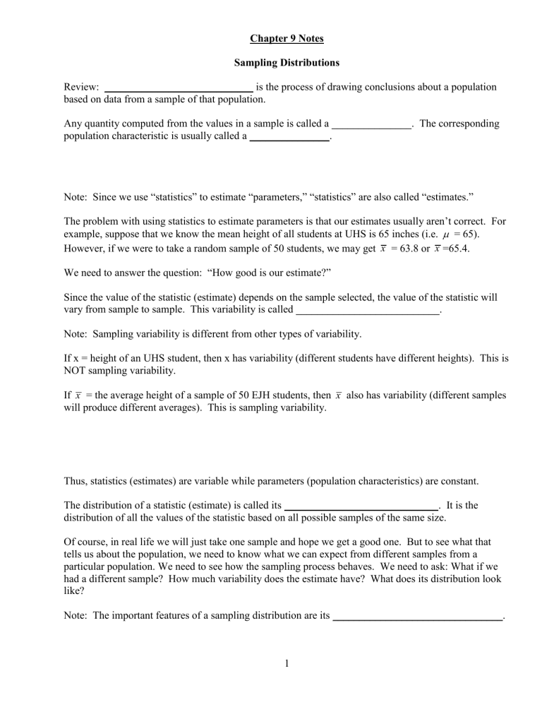
Chapter 9 Notes
Sampling Distributions
Review: ____________________________ is the process of drawing conclusions about a population
based on data from a sample of that population.
Any quantity computed from the values in a sample is called a _______________. The corresponding
population characteristic is usually called a _______________.
Note: Since we use “statistics” to estimate “parameters,” “statistics” are also called “estimates.”
The problem with using statistics to estimate parameters is that our estimates usually aren’t correct. For
example, suppose that we know the mean height of all students at UHS is 65 inches (i.e.  = 65).
However, if we were to take a random sample of 50 students, we may get x = 63.8 or x =65.4.
We need to answer the question: “How good is our estimate?”
Since the value of the statistic (estimate) depends on the sample selected, the value of the statistic will
vary from sample to sample. This variability is called ___________________________.
Note: Sampling variability is different from other types of variability.
If x = height of an UHS student, then x has variability (different students have different heights). This is
NOT sampling variability.
If x = the average height of a sample of 50 EJH students, then x also has variability (different samples
will produce different averages). This is sampling variability.
Thus, statistics (estimates) are variable while parameters (population characteristics) are constant.
The distribution of a statistic (estimate) is called its _____________________________. It is the
distribution of all the values of the statistic based on all possible samples of the same size.
Of course, in real life we will just take one sample and hope we get a good one. But to see what that
tells us about the population, we need to know what we can expect from different samples from a
particular population. We need to see how the sampling process behaves. We need to ask: What if we
had a different sample? How much variability does the estimate have? What does its distribution look
like?
Note: The important features of a sampling distribution are its ________________________________.
1
Suppose that our class is the population and we are taking samples of size 3 to estimate  = the true
mean hours of sleep for students last night.
x = Hours of sleep last night
x = average hours of sleep last night for 3 randomly selected students (sample mean)
The sampling distribution of x lists all possible values of x and how frequently they will occur.
Note: each possible statistic (range, median, proportion of males, etc.) has its own sampling distribution
2
A population of 5 people (and their score on the AP Exam) is shown below.
1. Adam (3)
2. Betty (4)
3. Carol (2)
4. Daniel (5)
5. Emily (4)
a. Suppose that a random sample of size 3 is chosen. List all 10 possible samples of size 3.
b. Graph the sampling distribution for the sample mean score, sample median score, and the proportion
of males for samples of size 3 from this population.
3
Modeling the Distribution of Sample Proportions
One of the major tasks of a statistician is to discover the proportion of individuals in a population who
possess a certain property or characteristic.
ex: p = proportion of US residents who are unemployed
ex: p = proportion of UHS students with at least one AP class
Unfortunately, without conducting a census, we will never know the true value of p, the
______________ _______________ (true proportion). Instead, statisticians will estimate p by taking a
sample and computing the __________________________________, p̂ .
p̂ =
number of "successes" in the sample x

sample size
n
Note: since x is the number of successes, x is a binomial random variable
Suppose that 22% of registered voters in Arizona are senior citizens (that is, p = .22). If we were to take
a sample of size 100 and find the sample proportion of senior citizens ( p̂ ), what values might we get?
What does the distribution of p̂ look like?
4
General Properties of the Sampling Distribution of a Sample Proportion:
Let p̂ be the proportion of successes in a random sample of size n from a population whose proportion
of successes is p. Denote the mean value of the p̂ distribution by  p̂ and the standard deviation of the
p̂ distribution by  p̂ . Then,
1.  p̂  p
pq
n
3. When n is large and p is not too close to 0 or 1, the sampling distribution of p̂ is approximately
normal.
2.  p̂ 
Conditions (for these properties to hold, the following must be true):
a. The data is from a random sample from population of interest
b. The sample is less than 10% of the population (so we can consider trials to be independent)
c. Large sample size: both np and nq are at least 10 (so the normal model is a good approximation
to the binomial)
Note: Rules 1 and 2 follow directly from the rules for binomial random variables.
 np
 pˆ  x 
p
n
n
npq

npq
pq
 pˆ  x 


2
n
n
n
n
Suppose that 43% of registered voters in Arizona are Democrats. What is the probability that there will
be less than 30% Democrats in a random sample of size 50?
5
If n = 50, what is the probability that the sample proportion will be within .05 of the true proportion?
How can we make this probability bigger?
Note: If the large sample size condition isn’t met (or if you just don’t like the normal distribution), you
can still use the binomial distribution. However, in later chapters we will need to use the normal
approximation so we will use it whenever we can from now on.
6
The Sampling Distribution of the Sample Mean
Another one of the major tasks of a statistician is to discover the mean (average) of a certain variable in
a population.
ex:  = mean income of US residents
ex:  = mean reduction in cholesterol for patients using a new drug
Unfortunately, without conducting a census, we will never know the true value of  , the
______________ _______________ (true mean). Instead, statisticians will estimate  by taking a
sample and computing the __________________________________, x .
General Properties of the Sampling Distribution of a Sample Mean ( x ):
Let x denote the mean of the observations in a random sample of size n from a population having mean
 x and standard deviation  x . Denote the mean value of the x distribution by  x and the standard
deviation of the x distribution by  x . Then, the following rules hold:
1.  x  x
2.  x 
x
n
3. When the population distribution of x is normal, the sampling distribution of x is also normal
for any size n.
4. Central Limit Theorem: When n is sufficiently large, the sampling distribution of x is well
approximated by a normal curve, even when the population is not normal.
Conditions:
a. The data is from a random sample from population of interest
b. The sample is less than 10% of population (so selections can be considered independent)
c. Large sample size (n > 30) OR distribution of population approximately normal (so distribution
of x can be considered approximately normal)
Note: Rules 1 and 2 come from the rules for combining independent random variables:
 x  x ... x   x   x  ...   x n   x
x 


 x
n
n
n
x 
  x  x ... x 
n

 x2   x2  ...   x2
n

n   x2
n

n   x2
 x2  x


n2
n
n
On the internet…
To explore other sampling distributions, try the following Applet: http://onlinestatbook.com/rvls.html
Choose “simulations/demo” and then “sampling distribution”
OR: http://interactivemaths.net/beta/
Go to Statistics and then to CLT.
7
Suppose that the weights of apples are approximately normally distributed with a mean of 200 grams
and a standard deviation of 35 grams.
a. What is the probability that if you choose one apple at random, its weight is at least 220 grams?
b. What is the probability that if you choose 25 apples at random, the average weight is at least 220 g?
Suppose that the population of residents of local town has a mean annual income of $50,000 and a
standard deviation of $35,000. If a random sample of 100 town residents is selected, what is the
probability that their sample mean is within $5000 of the true mean?
What will happen to this probability if we increase the sample size?
8