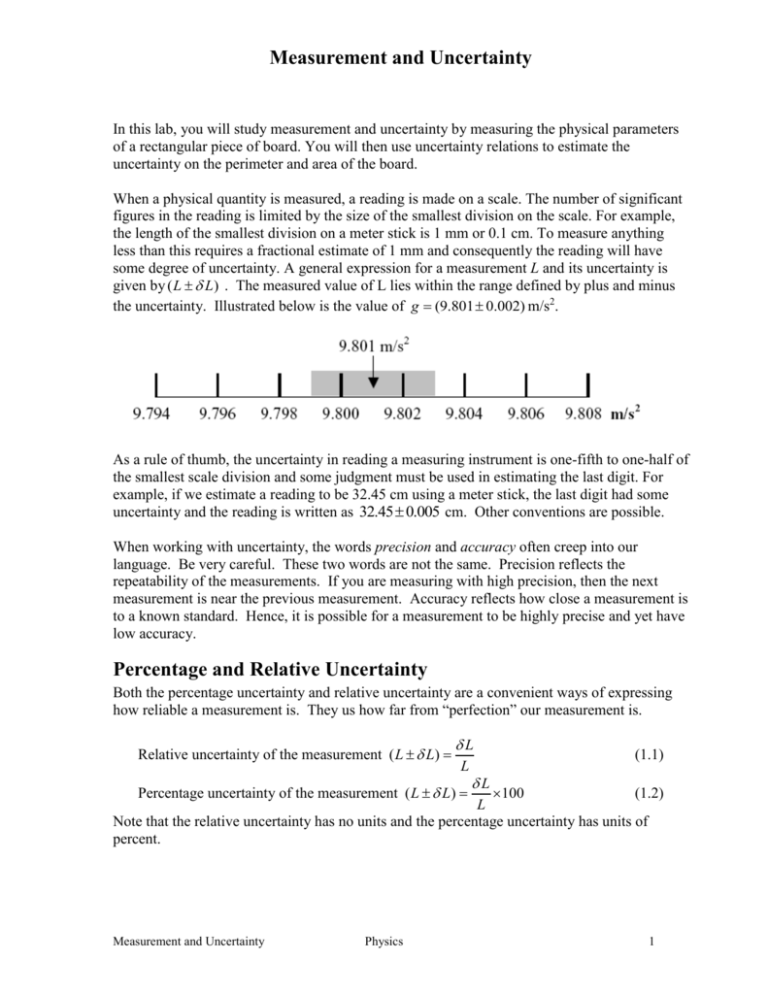
Measurement and Uncertainty
In this lab, you will study measurement and uncertainty by measuring the physical parameters
of a rectangular piece of board. You will then use uncertainty relations to estimate the
uncertainty on the perimeter and area of the board.
When a physical quantity is measured, a reading is made on a scale. The number of significant
figures in the reading is limited by the size of the smallest division on the scale. For example,
the length of the smallest division on a meter stick is 1 mm or 0.1 cm. To measure anything
less than this requires a fractional estimate of 1 mm and consequently the reading will have
some degree of uncertainty. A general expression for a measurement L and its uncertainty is
given by ( L   L) . The measured value of L lies within the range defined by plus and minus
the uncertainty. Illustrated below is the value of g  (9.801  0.002) m/s2.
As a rule of thumb, the uncertainty in reading a measuring instrument is one-fifth to one-half of
the smallest scale division and some judgment must be used in estimating the last digit. For
example, if we estimate a reading to be 32.45 cm using a meter stick, the last digit had some
uncertainty and the reading is written as 32.45  0.005 cm. Other conventions are possible.
When working with uncertainty, the words precision and accuracy often creep into our
language. Be very careful. These two words are not the same. Precision reflects the
repeatability of the measurements. If you are measuring with high precision, then the next
measurement is near the previous measurement. Accuracy reflects how close a measurement is
to a known standard. Hence, it is possible for a measurement to be highly precise and yet have
low accuracy.
Percentage and Relative Uncertainty
Both the percentage uncertainty and relative uncertainty are a convenient ways of expressing
how reliable a measurement is. They us how far from “perfection” our measurement is.
Relative uncertainty of the measurement ( L   L) 
L
L
Percentage uncertainty of the measurement ( L   L) 
(1.1)
L
100
(1.2)
L
Note that the relative uncertainty has no units and the percentage uncertainty has units of
percent.
Measurement and Uncertainty
Physics
1
Discrepancy
Consider two measurements, L and J and their respective uncertainties L and J. The two
measurements, L and J, agree when any value of L in the range define by ( L   L) are
identical to any value defined in the range ( J   J ) . When they do not share any values in
common, then we say that the measurements are discrepant. We can compute the discrepancy,
Z, between L and J as follows:
Z
LJ
 100
J
(1.3)
The discrepancy is particularly useful when the measurement J is a standard value that we are
attempting to determine experimentally. Hence, Z indicates how close our value of L is to the
standard value J.
We will often run experiments where we do not have a standard value of J. Instead, we will
have an expected value of J. In this case, the discrepancy is generally called the relative error
and is given by equation 1.2 above.
Averages or Means
We typically take measurements multiple times in our physics experiments to reduce random
error and hence we reduce the data to a mean or averaged value, called L . We sum all of the
separate measurements Li together and divide the total by the number of measurements n. n is
often called the sample size.
L
( L1  L2  ...Ln ) 1 n
  Li
n
n i 1
(1.4)
We can also calculate the deviation from the mean, labeled di , for each measurement Li.
di  Li  L
(1.5)
1 n
 di
n i 1
(1.6)
The average deviation is then given by
d
The average deviation could be used for our uncertainty; however, we generally use the
standard deviation or the standard deviation of the mean.
Standard Deviation
The sample standard deviation is a common way to mathematically describe the spread of a
data set for real world data sets we will encounter in our Physics labs. As the value of the
standard deviation decreases, then the precision of the data set increases. Of course, this says
nothing about the accuracy of the data. The sample standard deviation is labeled by the symbol
Measurement and Uncertainty
Physics
2
s, and is given by taking the square of the quotient of the sum of the squares of the average
deviation di (defined in equation 1.4) and the sample size minus 1 (n-1).
s
 d  d  ...d )
2
1
2
2
2
n
(n  1)
n

d
i 1
2
i
(n  1)
(1.7)
Standard Deviation of the Mean or Standard Error
When the final estimate of a measurement is an average of many individual measurements (the
general case for us in our Physics labs), then we do not compute the sample standard deviation
but rather the standard deviation of the mean (also called the standard error). As we make
more measurements, we expect the uncertainty of the average to get smaller and smaller. The
standard deviation of the mean or standard error is given the symbol , and is related to the
standard deviation, s, by

s
n
(1.8)
The standard error is always smaller than the sample standard deviation.
Propagation of Uncertainty
Whenever we combine measurements via mathematical operations (addition, subtract,
multiplication, and division) we need to properly handle the uncertainty. Doing so is called the
propagation of uncertainty and it can get rather involved as the mathematical operations get
more complicated. Instead of deriving the rules (using algebra or calculus), we will make use
of the end result.
Addition
The uncertainty of the sum of measurements L and J is the sum the uncertainty of L and the
uncertainty of J.
(1.9)
( L   L)  ( J   J )  ( L  J )  (  L   J )
Subtraction
The uncertainty of the subtraction of measurements L and J is the sum the uncertainty of L and
the uncertainty of J.
( L   L)  ( J   J )  ( L  J )  (  L   J )
(1.10)
Multiplication
The uncertainty of the product of measurements L and J is slightly more complicated than for
simple addition and subtraction. It is given by adding the relative uncertainties for L and J and
multiplying the resulting sum by the product of the two measurements.
Measurement and Uncertainty
Physics
3
  L  J 
( L   L)  ( J   J )  ( LJ ) 1  


J  
  L
(1.11)
You can obtain the percent uncertainty of the product by adding the percent uncertainties for L
and J.
Division
The uncertainty of the quotient of the measurements L and J is similar to the rule above for
multiplication. Simply replace the product (LJ) with the quotient (L/J).
( L   L)  L     L  J  
   1 


( J   J )  J    L
J  
(1.12)
You can obtain the percent uncertainty of the quotient by adding the percent uncertainties for L
and J.
Multiplication by a Constant
The uncertainty for multiplying a measurement and its uncertainty by a constant is given by
k ( L   L)  (kL)  k L
(1.13)
Note that this does not apply to changing units using standard conversion factors.
Square Root
The uncertainty for taking the square root of a measure and its uncertainty is given by
L
(1.14)
( L   L)  L 
2 L
You can obtain the percentage uncertainty of the square root L by dividing the percentage
uncertainty by two.
Logs
The uncertainty for a log requires a slightly different approach. Here we determine the
deviation between the log of the maximum L and the log of the minimum L. Half of this value
is the uncertainty.
log( L   L)  log( L)  0.5* log( L   L)  log( L   L)
(1.15)
The number of digits to display is the same as the number of significant figures in the original
value of L.
Trigonometric Functions
The uncertainty of a trig function follows an approach similar to that used with the log
function. Trigonometric function uncertainty is determined using radians not degrees.
sin( L   L)  sin( L)  0.5* sin( L   L)  sin( L   L)
Measurement and Uncertainty
Physics
(1.16)
4
The Lab
Read through the steps outline below and design an appropriate data table for your lab book.
All data should be taken in its native form with appropriate attention to uncertainty. Data
conversions should be carried out once the measurements are complete.
As we start the lab, we will create a series of measuring devices. At least one lucky person/lab
group will get an actual meter stick. The rest, well ….
Task 1
Step 1
Measure the length and width of your desk. Take multiple measurements. Estimate your
uncertainty. Did you use the end of the measuring device or did you start your measurement
past the end of the device? Average your results. Compute the deviation from the mean for
each measurement. Calculate the standard deviation and the standard error. How do they
differ? Which is larger? Does it make sense?
Step 2
Compute the perimeter of the board. Use your average measurements and express the
uncertainty for each average as the standard error. How will you handle the uncertainty for the
perimeter?
Step 3
Compute the area of the board. Use your average measurements and express the uncertainty
for each average as the standard error. How will you handle the uncertainty for the area?
Step 4
Be prepared to discuss your data with the class.
Task 2
Step 1
Determine the length of the side of the triangle labeled “a”. First measure it. Then determine
it using trig functions. How do you handle the uncertainty for these two measurements? Will
the results be the same? Should they be? Which is right?
Step 2
Be prepared to discuss your data with the class.
Measurement and Uncertainty
Physics
5