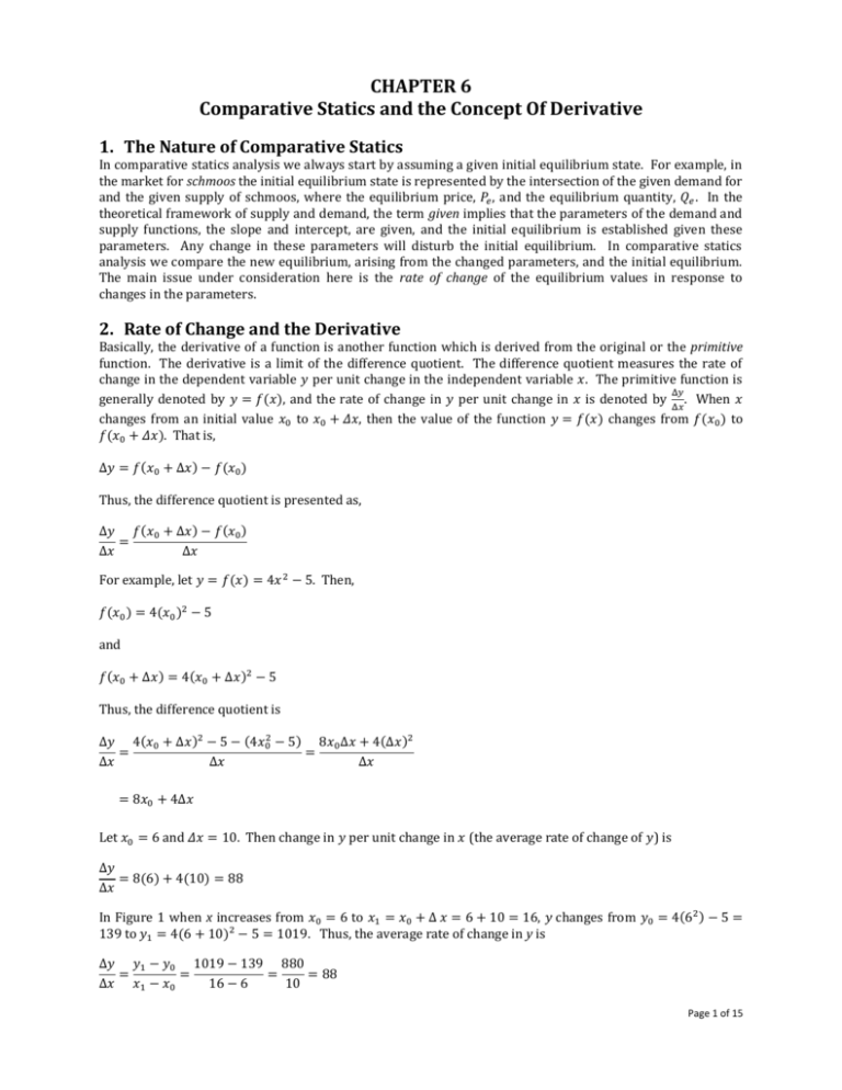
CHAPTER 6
Comparative Statics and the Concept Of Derivative
1. The Nature of Comparative Statics
In comparative statics analysis we always start by assuming a given initial equilibrium state. For example, in
the market for schmoos the initial equilibrium state is represented by the intersection of the given demand for
and the given supply of schmoos, where the equilibrium price, 𝑃𝑒 , and the equilibrium quantity, 𝑄𝑒 . In the
theoretical framework of supply and demand, the term given implies that the parameters of the demand and
supply functions, the slope and intercept, are given, and the initial equilibrium is established given these
parameters. Any change in these parameters will disturb the initial equilibrium. In comparative statics
analysis we compare the new equilibrium, arising from the changed parameters, and the initial equilibrium.
The main issue under consideration here is the rate of change of the equilibrium values in response to
changes in the parameters.
2. Rate of Change and the Derivative
Basically, the derivative of a function is another function which is derived from the original or the primitive
function. The derivative is a limit of the difference quotient. The difference quotient measures the rate of
change in the dependent variable 𝑦 per unit change in the independent variable 𝑥. The primitive function is
Δ𝑦
generally denoted by 𝑦 = 𝑓(𝑥), and the rate of change in 𝑦 per unit change in 𝑥 is denoted by . When 𝑥
Δ𝑥
changes from an initial value 𝑥0 to 𝑥0 + 𝛥𝑥, then the value of the function 𝑦 = 𝑓(𝑥) changes from 𝑓(𝑥0 ) to
𝑓(𝑥0 + 𝛥𝑥). That is,
∆𝑦 = 𝑓(𝑥0 + ∆𝑥) − 𝑓(𝑥0 )
Thus, the difference quotient is presented as,
Δ𝑦 𝑓(𝑥0 + ∆𝑥) − 𝑓(𝑥0 )
=
Δ𝑥
∆𝑥
For example, let 𝑦 = 𝑓(𝑥) = 4𝑥 2 − 5. Then,
𝑓(𝑥0 ) = 4(𝑥0 )2 − 5
and
𝑓(𝑥0 + ∆𝑥) = 4(𝑥0 + ∆𝑥)2 − 5
Thus, the difference quotient is
Δ𝑦 4(𝑥0 + ∆𝑥)2 − 5 − (4𝑥02 − 5) 8𝑥0 ∆𝑥 + 4(∆𝑥)2
=
=
Δ𝑥
∆𝑥
∆𝑥
Δ𝑦
= 8𝑥0 + 4∆𝑥
Δ𝑥
Let 𝑥0 = 6 and 𝛥𝑥 = 10. Then change in 𝑦 per unit change in 𝑥 (the average rate of change of 𝑦) is
Δ𝑦
= 8(6) + 4(10) = 88
Δ𝑥
In Figure 1 when x increases from 𝑥0 = 6 to 𝑥1 = 𝑥0 + ∆ 𝑥 = 6 + 10 = 16, 𝑦 changes from 𝑦0 = 4(62 ) − 5 =
139 to 𝑦1 = 4(6 + 10)2 − 5 = 1019. Thus, the average rate of change in y is
Δ𝑦 𝑦1 − 𝑦0 1019 − 139 880
=
=
=
= 88
Δ𝑥 𝑥1 − 𝑥0
16 − 6
10
Page 1 of 15
Figure 1
y
16, 1019
∆y = 880
∆x = 10
6, 139
x
Now, note what happens to the difference quotient as 𝛥𝑥 becomes smaller and smaller.
𝛥𝑥
10
5
2
0.5
0.1
0.01
0.001
0.0001
For 𝑥0 = 6
∆𝑦⁄∆𝑥 = 8𝑥0 + 4∆𝑥
88
68
56
50
48.4
48.04
48.004
48.0004
As Δ𝑥 gets smaller, the second term (4∆𝑥) on the right hand side of the difference quotient
∆𝑦⁄∆𝑥 = 8𝑥0 + 4∆𝑥
begins to disappear. In other words, as ∆𝑥 approaches zero, 8𝑥0 + 4∆𝑥 will approach the value 8𝑥0 = 8(6) =
48. Thus, for an infinitesimally small ∆𝑥 we may simply take the term 8𝑥0 on the right hand side of the
difference quotient as an approximation of ∆𝑦⁄∆𝑥 . In short, as ∆𝑥 approaches zero, ∆𝑦 ⁄∆𝑥 approaches 8𝑥0 .
In symbols, this fact is expressed by
𝐥𝐢𝐦
𝚫𝒚
∆𝒙→𝟎 𝚫𝒙
= 𝐥𝐢𝐦
∆𝒙→𝟎
𝒇(𝒙𝟎 + ∆𝒙) − 𝒇(𝒙𝟎 )
∆𝒙
𝚫𝒚
= 𝐥𝐢𝐦 𝟖𝒙𝟎 + 𝟒∆𝒙
∆𝒙→𝟎 𝚫𝒙
∆𝒙→𝟎
𝐥𝐢𝐦
lim
Δ𝑦
∆𝑥→0 Δ𝑥
= 8𝑥0
This reads as: “The limit of ∆𝑦⁄∆𝑥 as ∆𝑥 approaches zero is 8𝑥0 .” This limit is the derivative of the function
𝑦 = 𝑓(𝑥).
Page 2 of 15
In explaining the derivative of the function 𝑦 = 𝑓(𝑥) we have used the subscripted symbol 𝑥0 to point out the
fact that any change in 𝑥 must start from some specified value of 𝑥. Once the concept is explained, we
dispense with the subscript 0. The derivative, like the primitive function, is itself a function of 𝑥. To indicate
that it is a derivative function, it is usually expressed as 𝑦′ or 𝑓′(𝑥).
Also, since the derivative is simply a limit of the difference quotient ∆𝑦⁄∆𝑥, which measures a rate of change
in 𝑦, the derivative is also a measure of rate of change. But since the ∆𝑥 is infinitesimally small (∆𝑥 → 0), the
rate of change measured by the derivative is an instantaneous rate of change. Therefore, to distinguish
between the difference quotient and derivative as a measure of instantaneous rate of change we change the
symbols from ∆𝑦⁄∆𝑥 to 𝑑𝑦⁄𝑑𝑥 . Gathering all symbols representing the derivative of the function 𝑦 = 𝑓(𝑥),
we have
𝚫𝒚 𝒅𝒚
≡
≡ 𝒚′ ≡ 𝒇′(𝒙)
∆𝒙→𝟎 𝚫𝒙
𝒅𝒙
𝐥𝐢𝐦
Now referring back to the function used in explaining the derivative,
𝑦 = 𝑓(𝑥) = 4𝑥 2 − 5
𝒅𝒚
≡ 𝒚′ ≡ 𝒇′ (𝒙) = 𝟖𝒙
𝒅𝒙
Note that 8𝑥 is simply obtained by multiplying the coefficient of 𝑥 2 , 4, by the exponent of 𝑥 2 , 2, and then
raised 𝑥 to the exponent of 2 − 1 = 1.
𝑓 ′ (𝑥) = (2)4𝑥 2−1 = 8𝑥
2.1.
The Derivative and the Slope of the Curve of a Function
Consider the function 𝑦 = 𝑓(𝑥) = 4𝑥 2 − 5 again. In Figure 2 the points B and C on the curve represent the
values of y when 𝑥 is changed from the initial position 𝐴 (𝑥 = 6) to 16 (∆𝑥 = 10) and then to 13 (∆𝑥 = 7).
Note that as ∆𝑥 gets smaller, the line connecting the point 𝐴 to points 𝐵 and 𝐶 on the curve gets closer to the
curve. When ∆𝑥 is infinitesimally small around point 𝐴, this line will become tangent to the curve at that
point. We have defined the derivative 𝑑𝑦⁄𝑑𝑥 as the limit of ∆𝑦⁄∆𝑥 when ∆𝑥 → 0. Thus, the derivative of 𝑦
evaluated at point 𝐴 is the same as the slope of the line tangent to the curve at point 𝐴.
Figure 2
y
B
16, 1019
C
13, 671
D
13, 475
A
6, 139
x
Page 3 of 15
It was shown above that 𝑓′(𝑥) = 8𝑥. When 𝑥 = 6, then 𝑓′(𝑥) = 8𝑥. In the diagram the slope of the line
tangent at point 𝐴 is
𝚫𝒚 𝟒𝟕𝟓 − 𝟏𝟑𝟗
=
= 𝟒𝟖
𝚫𝒙
𝟏𝟑 − 𝟔
2.2. Rules of Differentiation
2.2.1. Constant-Function Rule
The function 𝑦 is a constant function when y is equal to a constant, 𝑦 = 𝑘. The derivative of a constant
function is always zero: 𝑦′ = 0. The graph of 𝑦 = 𝑘 is horizontal line with the vertical intercept of 𝑘. The
slope of the horizontal line is zero for all values of 𝑥. Thus the derivative of 𝑦 is zero for any value of 𝑥.
2.2.2. Power-Function Rule
A power-function is always of the form 𝒚 = 𝒇(𝒙) = 𝒙𝒏 . The exponent 𝒏 can be any real number. The
derivative of 𝒚 = 𝒙𝒏 takes the form of:
𝒚′ = 𝒇′(𝒙) = 𝒏𝒙𝒏−𝟏
Example 1
𝑦 = 𝑥5
𝑦′ =
𝑑𝑦
= 5𝑥 5−1 = 5𝑥 4
𝑑𝑥
𝑦 = 𝑥2
𝑦′ =
𝑑𝑦
= 2𝑥 2−1 = 2𝑥
𝑑𝑥
𝑦=𝑥
𝑦′ =
𝑑𝑦
= 𝑥 1−1 = 𝑥 0 = 1
𝑑𝑥
𝑦 = √𝑥 = 𝑥 1⁄2
𝑦′ =
𝑑𝑦 1 1⁄2−1 1 −1⁄2
1
= 𝑥
= 𝑥
=
𝑑𝑥 2
2
2√ 𝑥
𝑦′ =
𝑑𝑦
1
= (−1)𝑥 −1−1 = −𝑥 −2 = − 2
𝑑𝑥
𝑥
𝑦=
1
= 𝑥 −1
𝑥
If the power function includes a multiplicative constant 𝒄, so that
𝒇(𝒙) = 𝒄𝒙𝒏
the derivative is,
𝒇′ (𝒙) = 𝒄𝒏𝒙𝒏−𝟏
2.3. Derivatives of Two or More Functions of the Same Variable
Consider the two functions 𝒇(𝒙) = 𝒂𝒙𝒎 and 𝒈(𝒙) = 𝒃𝒙𝒏 . The derivative of the sum (difference) of the
functions is:
𝒇′ (𝒙) ± 𝒈′ (𝒙) = 𝒂𝒎𝒙𝒎−𝟏 ± 𝒃𝒏𝒙𝒏−𝟏
Example 2
𝒇(𝒙) = 𝟕𝒙𝟑
𝒈(𝒙) = 𝟒𝒙𝟑
𝒇’(𝒙) + 𝒈’(𝒙) = 𝟐𝟏𝒙𝟐 + 𝟏𝟐𝒙𝟐 = 𝟑𝟑𝒙𝟐
Page 4 of 15
𝒇’(𝒙) − 𝒈’(𝒙) = 𝟐𝟏𝒙𝟐 − 𝟏𝟐𝒙𝟐 = 𝟗𝒙𝟐
You can also combine the two primitive functions into one primitive function:
𝒚 = 𝒇(𝒙) + 𝒈(𝒙) = 𝟕𝒙𝟑 + 𝟒𝒙𝟑 = 𝟏𝟏𝒙𝟑
𝒚′ = 𝟑𝟑𝒙𝟐
𝒚 = 𝒇(𝒙) − 𝒈(𝒙) = 𝟕𝒙𝟑 − 𝟒𝒙𝟑 = 𝟑𝒙𝟑
𝒚′ = 𝟗𝒙𝟐
This rule can be extended to the sum of any number of functions. The exponents of the variable 𝒙 need not be
same.
2.3.1. Total Cost Function and Marginal Cost Function
In the theory of the firm we learned that the firm’s total variable cost (𝑻𝑽𝑪) is a function of the level of
output. We also learned that the firm’s marginal cost (𝑴𝑪) is the rate at which the firm’s cost changes per
each additional unit of output. Now we can discuss the firm’s 𝑴𝑪 as the derivative of the 𝑻𝑽𝑪.
Since cost is considered a function of output, then we let 𝒚 denote cost and 𝒙 the level of output. For a
numerical example, consider the following 𝑻𝑽𝑪 function. To simplify notation, let 𝑪 stand for 𝑻𝑽𝑪.
𝑪 = 𝒇(𝑸) = 𝑸𝟑 − 𝟏𝟐𝑸𝟐 + 𝟔𝟎𝑸
Although 𝑴𝑪 is defined in terms of a difference quotient ∆𝑪⁄∆𝑸, that is, change in variable cost per unit
increase in output, we can consider the rate of change in variable cost for very small changes in output. Thus,
we can look at 𝑴𝑪 as the derivative of the 𝑻𝑽𝑪 function.
𝑴𝑪 =
𝒅𝑪
= 𝟑𝑸𝟐 − 𝟐𝟒𝑸 + 𝟔𝟎
𝒅𝑸
Figure 3A and Figure 3B show the graphs of the primitive function (𝑪) and its derivative (𝑴𝑪).
Figure 3A
Total Variable Cost Function
0
Figure 3B
Marginal Cost Function
Q
Q
Note that if you add the total fixed cost to the 𝑻𝑽𝑪, it does not affect the marginal cost. Let 𝑻𝑭𝑪 = 𝟏𝟎𝟎, then
total cost (𝑻𝑪) is,
𝑻𝑪 = 𝑻𝑽𝑪 + 𝑻𝑭𝑪
Page 5 of 15
𝑻𝑪 = 𝒇(𝑸) = 𝑸𝟑 − 𝟏𝟐𝑸𝟐 + 𝟔𝟎𝑸 + 𝟏𝟎𝟎
𝑴𝑪 =
𝒅𝑻𝑪
= 𝟑𝑸𝟐 − 𝟐𝟒𝑸 + 𝟔𝟎
𝒅𝑸
Adding the fixed cost shifts the 𝑻𝑽𝑪 up by the amount of 𝑻𝑭𝑪. It does not affect the rate of change of the
function.
Figure 4
Total Cost Function
100
Q
2.3.2. Product Rule
Consider the two functions 𝒇(𝒙) = 𝒂𝒙𝒎 + 𝒄 and 𝒈(𝒙) = 𝒃𝒙𝒏 + 𝒅. The product of these two functions is,
𝒚 = 𝒇(𝒙)𝒈(𝒙) = (𝒂𝒙𝒎 + 𝒄)(𝒃𝒙𝒏 + 𝒅)
The derivative of the product is,
𝒅
[𝒇(𝒙)𝒈(𝒙)] = 𝒇′ (𝒙)𝒈(𝒙) + 𝒇(𝒙)𝒈′(𝒙)
𝒅𝒙
𝒅
[𝒇(𝒙)𝒈(𝒙)] = (𝒂𝒎𝒙𝒎−𝟏 )(𝒃𝒙𝒏 + 𝒅) + (𝒂𝒙𝒎 + 𝒄)(𝒃𝒏𝒙𝒏−𝟏 )
𝒚′ =
𝒅𝒙
Example 3
𝒚′ =
Let 𝒇(𝒙) = 𝟒𝒙𝟑 + 𝟓 and 𝒈(𝒙) = 𝟔𝒙𝟐 + 𝟐
𝒚 = (𝟒𝒙𝟑 + 𝟓)(𝟔𝒙𝟐 + 𝟐)
𝒚′ = (𝟏𝟐𝒙𝟐 )(𝟔𝒙𝟐 + 𝟐) + (𝟒𝒙𝟑 + 𝟓)(𝟏𝟐𝒙) = 𝟏𝟐𝟎𝒙𝟒 + 𝟐𝟒𝒙𝟐 + 𝟔𝟎𝒙
You may check the result by first multiplying out 𝒇(𝒙)𝒈(𝒙) and then taking the derivative.
𝒚 = 𝟐𝟒𝒙𝟓 + 𝟖𝒙𝟑 + 𝟑𝟎𝒙𝟐 + 𝟏𝟎
𝒚′ = 𝟏𝟐𝟎𝒙𝟒 + 𝟐𝟒𝒙𝟐 + 𝟔𝟎𝒙
2.3.3. Demand and Marginal Revenue in the Monopoly Model
In a typical supply/demand model in microeconomics the demand curve is represented by a linear downward
sloping curve. Even though in the model it is specified that, other things being equal (ceteris paribus),
quantity demanded of a good is a function of the price of that good, that is, 𝑸 = 𝒇(𝑷), contrary to the standard
mathematical convention, we put the price on the vertical axis and quantity on the horizontal axis.
Mathematically, however, the more accurate depiction of demand should be price being a function of
quantity: 𝑷 = 𝒇(𝑸)
Page 6 of 15
There is an important reason for stating the price on the vertical axis. Since a buyer’s or consumer’s demand
for a good is derived from the process of maximizing utility subject to a budget constraint, price of the
product reflects the amount the buyer is willing to pay for a given quantity. Price is the value the buyer places
on a given quantity. Thus, price becomes a function of quantity, rather than the other way around. The law of
diminishing marginal utility provides that as more of the good is consumed, the utility of (value placed on, or
the price the consumer is willing to pay for) each additional unit decreases.
In the monopoly model, the monopolist, as a single seller faces the whole market demand curve. Thus to
increase sales, to have buyers buy more of the product, the monopolist must lower its price.
In the theory of the firm, the firm (competitive or otherwise) maximizes profit where marginal revenue
equals marginal cost. This aspect of the firm’s behavior will be discussed later. For now we are interested in
the marginal revenue side of the profit maximizing criterion.
The firm’s marginal revenue function is derived from its demand function. To explain, let’s start with the
demand function
𝑷 = 𝒇(𝑸)
The firm’s total revenue (𝑹) is determined as the product of the price (𝑷) times the quantity (𝑸) sold.
𝑹 = 𝑷𝑸 = 𝒇(𝑸)𝑸
Marginal revenue (𝑴𝑹) is the rate of change in 𝑹 per each additional unit sold. For very small changes in 𝑸,
𝑴𝑹 is the derivative of the total revenue function.
𝑴𝑹 =
𝒅𝑹
= 𝒇′ (𝑸)𝑸 + 𝒇(𝑸)
𝒅𝑸
To recognize the relationship between the demand function and the 𝑴𝑹 function, let’s obtain the difference
between the two functions
𝑴𝑹 − 𝑷 = 𝒇′(𝑸)𝑸 + 𝒇(𝑸) − 𝒇(𝑸) = 𝒇′(𝑸)𝑸
Note that in the product term 𝒇′(𝑸)𝑸, 𝑸 (quantity of output) is always a positive value. However, since the
law of demand provides for an inverse relation between price and quantity, 𝒅𝑷⁄𝒅𝑸 = 𝒇′ (𝑸) < 𝟎. Thus,
𝑴𝑹 − 𝑷 = 𝒇′ (𝑸)𝑸 < 𝟎
Since 𝑴𝑹 − 𝑷 < 𝟎, then 𝑴𝑹 < 𝑷. This means that the 𝑴𝑹 function (curve) is always below the demand
function (curve).
To explore further the relationship between 𝑴𝑹 and 𝑷, let’s use the general linear demand function of the
form,
𝑷 = 𝒂 − 𝒃𝑸
Then the total revenue function 𝑹 = 𝑷𝑸 is
𝑹 = (𝒂 − 𝒃𝑸)𝑸
𝑴𝑹 function is thus,
𝑴𝑹 =
𝒅𝑹
= −𝒃𝑸 + (𝒂 − 𝒃𝑸) = 𝒂 − 𝟐𝒃𝑸
𝒅𝑸
Page 7 of 15
We can also write 𝑹 by multiplying out (𝒂 − 𝒃𝑸) and 𝑸 and then find 𝑴𝑹
𝑹 = 𝒂𝑸 − 𝒃𝑸𝟐
𝑴𝑹 = 𝒂 − 𝟐𝒃𝑸
Now we can see that he slope of the 𝑴𝑹 curve, – 𝟐𝒃 in 𝑴𝑹 = 𝒂 − 𝟐𝒃𝑸, is twice that of the demand curve 𝑷 =
𝒂 − 𝒃𝑸.
Example 4
Determine the MR function from the following demand function.
𝑷 = 𝟐𝟎 − 𝟐𝑸
𝑹 = (𝟐𝟎 − 𝟐𝑸)𝑸 = 𝟐𝟎𝑸 − 𝟐𝑸𝟐
𝑴𝑹 = 𝟐𝟎 − 𝟒𝑸
Figure 5
Demand Function and the MR Function
P
P = 20 − 2Q
MR = 20 − 4Q
Q
2.3.4. The Product Rule Extended

𝒚 = 𝒇𝟐 (𝒙)
𝒚 = 𝒇(𝒙)𝒇(𝒙)
𝒚′ = 𝒇′ (𝒙)𝒇(𝒙) + 𝒇(𝒙)𝒇′(𝒙)
𝒚′ = 𝟐𝒇(𝒙)𝒇′(𝒙)
Example 5
𝒚 = (𝟑𝒙𝟐 + 𝟒𝒙 + 𝟏)𝟐
𝒚′ = 𝟐(𝟑𝒙𝟐 + 𝟒𝒙 + 𝟏)(𝟔𝒙 + 𝟒)
Page 8 of 15

𝒚 = 𝒇𝒏 (𝒙)
𝒚′ = 𝒏𝒇𝒏−𝟏 (𝒙)𝒇′ (𝒙)
Example 6
𝑦 = (5𝑥 3 + 4𝑥 2 + 8𝑥)4
𝑦 ′ = 4(5𝑥 3 + 4𝑥 2 + 8𝑥)3 (15𝑥 2 + 8𝑥 + 8)

𝑦=
1
= 𝑓 −1 (𝑥)
𝑓(𝑥)
𝑦 ′ = −𝑓 −2 𝑓 ′ (𝑥) = −
𝑓′(𝑥)
𝑓 2 (𝑥)
Example 7
𝑦=
1
= (3𝑥 2 + 4𝑥 + 1)−1
3𝑥 2 + 4𝑥 + 1
𝑦 ′ = −(3𝑥 2 + 4𝑥 + 1)−2 (6𝑥 + 4)
𝑦′ = −
(6𝑥 + 4)
+ 4𝑥 + 1)2
(3𝑥 2
2.3.5. Quotient Rule
𝑦=
𝑓(𝑥)
= 𝑓(𝑥)𝑔−1 (𝑥)
𝑔(𝑥)
First, the derivative of 𝑓(𝑥), 𝑓′(𝑥), times 𝑔−1 (𝑥) is:
𝑓′(𝑥)𝑔−1 (𝑥)
Next, the derivative of the second term 𝑔−1 (𝑥), −𝑔−2 (𝑥)𝑔′(𝑥), times 𝑓(𝑥) is:
−𝑔−2 (𝑥)𝑔′(𝑥)𝑓(𝑥)
Using the product rule, we have
𝑦 ′ = 𝑓′(𝑥)𝑔−1 (𝑥) − 𝑔−2 (𝑥)𝑔′(𝑥)𝑓(𝑥)
𝑦 ′ = 𝑔−1 (𝑥)[𝑓′(𝑥) − 𝑔−1 (𝑥)𝑔′(𝑥)𝑓(𝑥)]
𝑦′ =
1
𝑓(𝑥)𝑔′(𝑥)
[𝑓′(𝑥) −
]
𝑔(𝑥)
𝑔(𝑥)
𝑦′ =
𝑓 ′ (𝑥)𝑔(𝑥) − 𝑓(𝑥)𝑔′(𝑥)
𝑔2 (𝑥)
Page 9 of 15
Example 8
𝑦=
6𝑥 2 − 4𝑥 + 2
2𝑥 + 1
𝑦′ =
(12𝑥 − 4)(2𝑥 + 1) − (6𝑥 2 − 4𝑥 + 2)(2)
(2𝑥 + 1)2
𝑦′ =
12𝑥 2 + 12𝑥 − 8
(2𝑥 + 1)2
2.3.6. Relationship Between Marginal Cost and Average Cost Functions
To explain the relationship between the 𝑀𝐶 function and the 𝐴𝐶 function let’s start with the cost function in
Section 2.3.1. To simplify the explanation of the relationship we will leave the fixed cost out of the picture by
assuming 𝑇𝐹𝐶 = 0.
𝐶 = 𝑓(𝑄) = 𝑄3 − 12𝑄2 + 60𝑄
The MC function and AC function are, respectively,
𝑀𝐶 =
𝑑𝐶
= 3𝑄2 − 24𝑄 + 60
𝑑𝑄
𝐴𝐶 =
𝐶
= 𝑄2 − 12𝑄 + 60
𝑄
Figure 6 shows the graphs of these functions.
Figure 6
Marginal Cost and Average Cost
MC and AC
MC
AC
6
Q
To explain how the behavior of MC and AC are related, let’s obtain the derivative of the AC function.
𝑑𝐴𝐶
= 2𝑄 − 12
𝑑𝑄
Page 10 of 15
The derivative of AC shows the rate of change in AC per each (very small) addition to output. Now consider
the following table. Note that up to the output level 𝑄 = 6 average cost is decreasing. That is, 𝑑𝐴𝐶 ⁄𝑑𝑄 < 0.
At this output range 𝑀𝐶 < 𝐴𝐶. At 𝑄 = 6, 𝑑𝐴𝐶 ⁄𝑑𝑄 = 0 and 𝑀𝐶 = 𝐴𝐶. Beginning with 𝑄 = 7, 𝑑𝐴𝐶 ⁄𝑑𝑄 > 0and
𝑀𝐶 > 𝐴𝐶.
Q
𝑑𝐴𝐶 ⁄𝑑𝑄
MC
AC
1
-10
39
49
2
-8
24
40
3
-6
15
33
4
-4
12
28
5
-2
15
25
6
0
24
24
7
2
39
25
8
4
60
28
9
6
87
33
10
8
120
40
This relationship in numbers can also be shown mathematically using the quotient rule.
𝑑𝐴𝐶
𝑑 𝑓(𝑄)
𝑓′(𝑄)𝑄 − 𝑓(𝑄) 1 ′
𝑓(𝑄)
=
(
)=
= [𝑓 (𝑄) −
]
2
𝑑𝑄
𝑑𝑄 𝑄
𝑄
𝑄
𝑄
𝑑𝐴𝐶 1
= (𝑀𝐶 − 𝐴𝐶)
𝑑𝑄
𝑄
Given that 𝑄 > 0,
𝑑𝐴𝐶
< 0 if 𝑀𝐶 < 𝐴𝐶
𝑑𝑄
𝑑𝐴𝐶
= 0 if 𝑀𝐶 = 𝐴𝐶
𝑑𝑄
𝑑𝐴𝐶
> 0 if 𝑀𝐶 > 𝐴𝐶
𝑑𝑄
3. Rules of Differentiation Involving Functions of Different Variables
Here we deal with two or more functions, each with a distinct independent variable.
3.1. Chain Rule
Consider a differentiable function 𝑧 = 𝑓(𝑦), where 𝑦 is in turn a differentiable function of another variable 𝑥,
𝑦 = 𝑓(𝑥). Chain rule provides the rule to find the derivative of 𝑧 with respect to 𝑥.
𝑑𝑧 𝑑𝑧 𝑑𝑦
=
= 𝑓 ′ (𝑦)𝑓 ′ (𝑥)
𝑑𝑥 𝑑𝑦 𝑑𝑥
Page 11 of 15
Example 9
Let 𝑧 = 5𝑦 2 + 3𝑦, and 𝑦 = 6𝑥 + 4. Find 𝑑𝑧⁄𝑑𝑥 .
𝑑𝑧
= 𝑓 ′ (𝑦) = 10𝑦 + 3
𝑑𝑦
𝑑𝑦
= 𝑓 ′ (𝑥) = 6
𝑑𝑥
𝑑𝑧
= 𝑓 ′ (𝑦)𝑓 ′ (𝑥) = (10𝑦 + 3)(6) = 60𝑦 + 18
𝑑𝑥
3.1.1. Marginal Revenue Product
In the theory of the firm, the profit maximizing amount of variable input is where the marginal revenue
product (or value of marginal product) is equal to the wage rate. The 𝑀𝑅𝑃𝐿 (or 𝑉𝑀𝑃𝐿 ) is the additional
(marginal) revenue gained from the output of the additional unit (marginal product) of variable input hired.
Let 𝑃 stand for the price of the product. The firm’s total revenue is
𝑅 = 𝑓(𝑄)
From which we obtain the marginal revenue function,
𝑀𝑅 = 𝑓 ′ (𝑄) =
𝑑𝑅
𝑑𝑄
The total product, defined as a function of variable input 𝐿, is
𝑄 = 𝑔(𝐿)
From which we obtain the marginal product function,
𝑀𝑃𝐿 = 𝑔′ (𝐿) =
𝑑𝑄
𝑑𝐿
Using chain rule, 𝑀𝑅𝑃𝐿 is then obtained as the product of marginal revenue times marginal product. Thus,
𝑀𝑅𝑃𝐿 =
𝑑𝑅 𝑑𝑅 𝑑𝑄
=
= 𝑓 ′ (𝑄)𝑔′ (𝐿) = 𝑀𝑅 ∙ 𝑀𝑃𝐿
𝑑𝐿 𝑑𝑄 𝑑𝐿
3.2. Inverse Function Rule
For a function 𝑦 = 𝑓(𝑥), the inverse function rule of differentiation provides that,
𝑑𝑥
1
=
𝑑𝑦 𝑑𝑦⁄𝑑𝑥
Note however that for the inverse function rule to apply the inverse of the primitive function 𝑦 = 𝑓(𝑥) must
exist. The inverse is denoted by 𝑥 = 𝑓 −1 (𝑦). Not all primitive functions have an inverse. Remember that the
functional relationship between 𝑥 and 𝑦, that is 𝑦 = 𝑓(𝑥), requires that for each value of the independent
variable 𝑥 there exists only one corresponding value 𝑦.
To maintain the functional relationship when 𝑥 is the dependent and 𝑦 the independent variable, that is 𝑥 =
𝑓(𝑦), for each value of y there must be only one corresponding value 𝑥. For this to hold, the original function
must be monotonic. The monotonic condition requires that the function must be either increasing or
Page 12 of 15
decreasing for all successively increasing values of 𝑥. The function may not contain a maximum or a
minimum.
Examples of monotonic functions in economics include the short-run cost function 𝐶 = 𝑓(𝑄) and the shortrun production function 𝑄 = 𝑔(𝐿).
Consider the graphs of the following functions.
Total cost:
Total product:
𝐶 = 𝑓(𝑄) = 𝑄3 − 12𝑄2 + 60𝑄
𝑄 = 𝑔(𝐿) = 15𝐿2 − 𝐿3
The graph of each function indicate that they are both monotonic.
Figure 7A
Total Cost Function
𝐶 = 𝑓(𝑄) = 𝑄3 − 12𝑄2 + 60𝑄
Figure 7B
Total Product Function
𝑄 = 𝑔(𝐿) = 15𝐿2 − 𝐿3
g(L)
f(Q)
Q
L
Although finding the inverse of the above functions, that is, 𝑄 = 𝑓 −1 (𝐶) and 𝐿 = 𝑔−1 (𝑄) is quite impractical,
we can find the derivatives of the inverse functions easily using the inverse function rule.
𝑑𝑄
1
1
=
=
2
𝑑𝐶 𝑑𝐶 ⁄𝑑𝑄 3𝑄 − 24𝑄 + 60
𝑑𝐿
1
1
=
=
𝑑𝑄 𝑑𝑄 ⁄𝑑𝐿 30𝑄 − 3𝑄2
4. Partial Derivatives
In many situations in economics we find a dependent variable a function of more than one independent
variable. For example, in a production function, output can be a function of more than one input. The typical
example is,
𝑄 = 𝑓(𝐾, 𝐿)
where the level of output is a function of the combination of two inputs capital (𝐾) and labor (𝐿).
Multivariable functions are encountered extensively in econometric analysis.
To explain partial derivatives, consider the general multivariate functional form,
𝑦 = 𝑓(𝑥1 , 𝑥2 , ⋯ , 𝑥𝑛 )
Page 13 of 15
Here the independent variables 𝑥𝑖 are all independent of one another. This means that variations in one
variable does not affect the others; one can change the value of one variable, while holding the other variables
constant. By changing the values of one variable, while holding others constant, we can observe the rate of
change in 𝑦 per unit change in the varied variable.
∆𝑦
𝑓(𝑥1 + ∆𝑥1 , 𝑥2 , ⋯ , 𝑥𝑛 ) − 𝑓(𝑥1 , 𝑥2 , ⋯ , 𝑥𝑛 )
=
∆𝑥1
∆𝑥1
The partial derivative of 𝑦 with respect of 𝑥1 , denoted by 𝑓1 or
𝑓1 =
𝝏𝒚
𝝏𝒙𝟏
, is defined as
𝜕𝑦
∆𝑦
= 𝐥𝐢𝐦
𝜕𝑥1 ∆𝑥1→0 ∆𝑥1
Example 10
Find the partial derivatives
𝝏𝒚
𝝏𝒚
and
𝝏𝒙𝟏
𝝏𝒙𝟐
of
𝑦 = 3𝑥12 + 𝑥1 𝑥2 + 4𝑥22
To find
𝜕𝑦
𝜕𝑥1
, you must treat 𝑥2 like any other constant in the function. Thus,
𝜕𝑦
= 𝑓1 = 6𝑥1 + 𝑥2
𝜕𝑥1
Similarly,
𝜕𝑦
= 𝑓2 = 𝑥1 + 8𝑥2
𝜕𝑥2
Example 11
Find the partial derivatives of,
𝑦 = (𝑥1 + 4)(3𝑥1 + 2𝑥2 )
To observe the process of partial differentiation clearly, denote 𝑥2 = 𝑘 as a constant for finding
𝜕𝑦
𝜕𝑥1
.
𝑦 = (𝑥1 + 4)(3𝑥1 + 2𝑘)
𝜕𝑦
= (1)(3𝑥1 + 2𝑘) + 3(𝑥1 + 4)
𝜕𝑥1
𝜕𝑦
= 6𝑥1 + 2𝑘 + 12 = 6𝑥1 + 2𝑥2 + 12
𝜕𝑥1
Similarly, let 𝑥1 = 𝑘 for finding
𝜕𝑦
𝜕𝑥2
𝑦 = (𝑘 + 4)(3𝑘 + 2𝑥2 )
Page 14 of 15
𝜕𝑦
= 2(𝑘 + 4) = 2(𝑥1 + 4)
𝜕𝑥2
Example 12
Find the partial derivatives of
𝑦=
3𝑥1 − 2𝑥2
𝑥12 + 3𝑥2
𝜕𝑦
3(𝑥12 + 3𝑥2 ) − 2𝑥1 (3𝑥1 − 2𝑥2 ) −3𝑥12 + 4𝑥1 𝑥2 + 9𝑥2
=
=
(𝑥12 + 3𝑥2 )2
(𝑥12 + 3𝑥2 )2
𝜕𝑥1
𝜕𝑦
−2(𝑥12 + 3𝑥2 ) − 3(3𝑥1 − 2𝑥2 ) −𝑥1 (2𝑥1 + 9)
=
=
(𝑥12 + 3𝑥2 )2
(𝑥12 + 3𝑥2 )2
𝜕𝑥2
Page 15 of 15