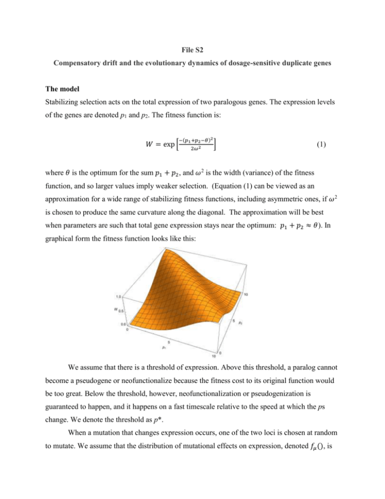
File S2
Compensatory drift and the evolutionary dynamics of dosage-sensitive duplicate genes
The model
Stabilizing selection acts on the total expression of two paralogous genes. The expression levels
of the genes are denoted p1 and p2. The fitness function is:
𝑊 = exp [
−(𝑝1 +𝑝2 −𝜃)2
2𝜔 2
]
(1)
where 𝜃 is the optimum for the sum 𝑝1 + 𝑝2, and 𝜔2 is the width (variance) of the fitness
function, and so larger values imply weaker selection. (Equation (1) can be viewed as an
approximation for a wide range of stabilizing fitness functions, including asymmetric ones, if 𝜔2
is chosen to produce the same curvature along the diagonal. The approximation will be best
when parameters are such that total gene expression stays near the optimum: 𝑝1 + 𝑝2 ≈ 𝜃). In
graphical form the fitness function looks like this:
We assume that there is a threshold of expression. Above this threshold, a paralog cannot
become a pseudogene or neofunctionalize because the fitness cost to its original function would
be too great. Below the threshold, however, neofunctionalization or pseudogenization is
guaranteed to happen, and it happens on a fast timescale relative to the speed at which the ps
change. We denote the threshold as p*.
When a mutation that changes expression occurs, one of the two loci is chosen at random
to mutate. We assume that the distribution of mutational effects on expression, denoted 𝑓𝜇 (), is
2
normal with mean 0 and variance 𝜎𝑚
. The probability that a mutation with an effect 𝛿 on either
p1 or p2 fixes is denoted 𝑃𝑓𝑖𝑥 (𝛿). There is a probability 𝜇 per generation that a mutation affecting
expression will occur at each of the two gene copies at each of the two paralogs. The waiting
time until the next mutation appears in the population is exponentially-distributed with mean
1/(4𝑁𝜇). The evolutionary dynamics therefore proceed as a random walk in p1 and p2.
A diffusion approximation
It is useful to work in terms of the sum A and the difference D in expression at the two loci:
𝐴 = 𝑝1 + 𝑝2
𝐷 = 𝑝1 − 𝑝2
(2)
There are two reasons for this change of variables. Stabilizing selection acts on A but is
indifferent to D, and that fact simplifies the derivation below. Second, our data are on D (see File
S3), and so this parameterization focuses our attention in the model on the quantity of empirical
interest.
In the absence of boundary conditions (that is, with no neofunctionalization), the density
function for A and D can be written as the product of independent density functions:
𝑓𝐴,𝐷 = 𝑓𝐴 (𝐴)𝑓𝐷 (𝐷)
(3)
That relation also holds approximately when neofunctionalization does happen if stabilizing
selection is strong relative to drift. Then the value of A will stay very close to its optimal value.
The evolutionary dynamics then lie (almost) along a single dimension in which 𝐴 = 𝜃 and the
difference in expression, D diverges with time. This is the key approximation to what follows.
We will therefore assume this situation holds, and proceed to develop a partial differential
equation (PDE) for the density function fD(). Simulations described in File S1 validate the
accuracy of this approximation over the parameter values of biological interest to us. The PDE
for D follows that of simple Brownian motion:
1
𝜕𝑡 𝑓𝐷 = 2 𝜎𝐷2 𝜕𝐷,𝐷 𝑓𝐷
(4)
The diffusion coefficient 𝜎𝐷2 determines the evolutionary rate at which D will diverge in the
paralogs.
Calculating the diffusion coefficient
The diffusion coefficient is defined as the instantaneous rate of increase in the variance of D, the
difference of expression in the paralogs. We calculate that rate as
2
𝜎𝐷2 = ∫(𝛿 − 𝛿 ̅) [4𝑁𝜇𝑓𝜇 (𝛿)]𝑃𝑓𝑖𝑥 (𝛿)𝑑𝛿
(5)
where 𝛿 ̅ is the mean effect of mutations that fix, which is approximately 0. The term in square
brackets represents the number of new mutations with effect 𝛿 entering the population each
generation. 𝑃𝑓𝑖𝑥 (𝛿) is the probability that a mutation with effect 𝛿 fixes, for which we use
Kimura’s (1964) approximation:
𝑃fix (𝛿) =
1−exp[−2𝑠(𝛿)]
1−exp[−4𝑁𝑠(𝛿)]
(6)
Here 𝑠(𝛿) is the relative fitness of a mutation with an effect 𝛿 on expression:
𝑊(𝛿)
𝑠(𝛿) ≈ 𝑊(0) − 1
−𝛿 2
≈ exp [2𝜔2 ] − 1 ≈
(7)
−𝛿 2
(8)
2𝜔 2
Equation (7) makes use of the earlier assumption that selection is sufficiently strong relative to
drift that A is typically very close to 𝜃.
Combining these expressions gives us
𝜎𝐷2 =
4𝑁𝜇
√2𝜋𝜎𝑚
−𝛿 2
∫ 𝛿 2 exp [2𝜎2 ] (
𝑚
𝛿2
exp[ 2 ]−1
𝜔
exp[
) 𝑑𝛿
2𝛿2 𝑁
]−1
𝜔2
(9)
That integral cannot be solved analytically. We can, however, determine its value using the
following combination of analytic and numerical arguments. The probability that a mutation
fixes is close to that for a neutral mutation (= 1/2N) if the magnitude of its selection coefficient is
sufficiently small, while the probability becomes negligible if the selection coefficient is larger
than that. From basic population genetics, we know that this critical value for the selection
coefficient is c/2N, where c is an unknown constant that is approximately equal to 1 (Crow and
Kimura, 1970). Using 𝛿 ∗ to denote the mutational effect corresponding to that selection
coefficient, we find from Equation (8) that
𝑐𝜔 2
𝛿∗ = √
𝑁
.
(10)
Now assume that the average size of mutational effects is much greater than 𝛿 ∗ , in which case
𝑓𝜇 (𝛿) ≈ 𝑓𝜇 (0) for −𝛿 ∗ < 𝛿 < 𝛿 ∗ . Equation (9) for the diffusion coefficient is now
𝛿∗
1
𝜎𝐷2 ≈ 4𝑁𝜇 ∫−𝛿∗ 𝛿 2 𝑓𝜇 (𝛿) (2𝑁) 𝑑𝛿
≈ 𝑘𝜎
𝜇𝜔 3
𝑚𝑁
3/2
,
(11)
(12)
where k is a numerical constant that is independent of all of the model’s parameters.
The last element needed is the value of k. While we could resort to further analytic
approximations, we chose to determine the value for k using stochastic simulations. We
simulated a random walk in p1 and p2 (or equivalently, in A and D) in the absence of absorbing
boundaries at p = p* and 𝜃 − 𝑝∗ . We calculated the variance among replicate simulations at
time t and fit k using the fact that under Equation (4) we expect
𝑉𝑎𝑟[𝐷] = 𝜎𝐷2 𝑡.
(13)
We find that k ≈ 1.543. We verified that consistent results are obtained from simulations using
2
different values for 𝜇, 𝜔2 , 𝜎𝑚
, and N so long as the resulting value for 𝜎𝐷2 as given by Equation
(12) is unaltered.
References
Crow, J. F. and M. Kimura, 1970 An Introduction to Population Genetics. New York: Harper &
Row.