Appendix to “The Bayesian Change Point and Variable Selection Algorithm: Application to the
δ18O Proxy Record of the Plio-Pleistocene” published in the Journal of Computational and
Graphical Statistics
Authors:
Eric Ruggieri, Duquesne University
Charles E. Lawrence, Brown University
Appendix A: The Bayesian Change Point and Variable Selection Algorithm
The Bayesian Change Point Algorithm updated to include the EBIR variable selection procedure is
described below. The dependence on X has been suppressed. Steps that differ from the original
algorithm are indicated with a ‘*’.
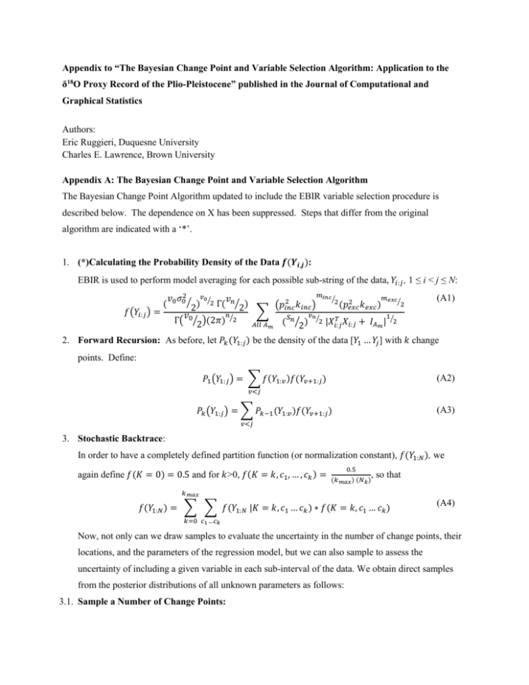
1. (*)Calculating the Probability Density of the Data 𝒇(𝒀𝒊,𝒋 ):
EBIR is used to perform model averaging for each possible sub-string of the data, 𝑌𝑖:𝑗 , 1 ≤ i < j ≤ N:
𝑚𝑖𝑛𝑐
𝑚𝑒𝑥𝑐⁄
⁄2 2
𝑣0 𝜎02⁄ 𝑣0⁄2 𝑣𝑛
2
2
)
Γ( ⁄2)
𝑘𝑖𝑛𝑐 )
(𝑝𝑒𝑥𝑐 𝑘𝑒𝑥𝑐 )
(𝑝𝑖𝑛𝑐
2
𝑓(𝑌𝑖:𝑗 ) =
∑
𝑛
𝑣
𝑣
𝑛⁄
1
𝑠𝑛
Γ( 0⁄2)(2𝜋) ⁄2
2 |𝑋 𝑇 𝑋𝑖:𝑗 + 𝐼𝐴 | ⁄2
𝐴𝑙𝑙 𝐴𝑚 ( ⁄2)
𝑖:𝑗
𝑚
(
(A1)
2. Forward Recursion: As before, let 𝑃𝑘 (𝑌1:𝑗 ) be the density of the data [𝑌1 … 𝑌𝑗 ] with 𝑘 change
points. Define:
𝑃1 (𝑌1:𝑗 ) = ∑ 𝑓(𝑌1:𝑣 )𝑓(𝑌𝑣+1:𝑗 )
(A2)
𝑣<𝑗
𝑃𝑘 (𝑌1:𝑗 ) = ∑ 𝑃𝑘−1 (𝑌1:𝑣 )𝑓(𝑌𝑣+1:𝑗 )
(A3)
𝑣<𝑗
3. Stochastic Backtrace:
In order to have a completely defined partition function (or normalization constant), 𝑓(𝑌1:𝑁 ), we
again define 𝑓(𝐾 = 0) = 0.5 and for 𝑘>0, 𝑓(𝐾 = 𝑘, 𝑐1 , … , 𝑐𝑘 ) =
0.5
,
(𝑘𝑚𝑎𝑥 ) (𝑁𝑘 )
so that
𝑘𝑚𝑎𝑥
𝑓(𝑌1:𝑁 ) = ∑ ∑ 𝑓(𝑌1:𝑁 |𝐾 = 𝑘, 𝑐1 … 𝑐𝑘 ) ∗ 𝑓(𝐾 = 𝑘, 𝑐1 … 𝑐𝑘 )
(A4)
𝑘=0 𝑐1 …𝑐𝑘
Now, not only can we draw samples to evaluate the uncertainty in the number of change points, their
locations, and the parameters of the regression model, but we can also sample to assess the
uncertainty of including a given variable in each sub-interval of the data. We obtain direct samples
from the posterior distributions of all unknown parameters as follows:
3.1. Sample a Number of Change Points:
𝑓(𝐾 = 𝑘|𝑌1:𝑁 ) =
𝑃𝑘 (𝑌1:𝑁 )𝑓(𝑐1 , … , 𝑐𝑘 |𝐾 = 𝑘)𝑓(𝐾 = 𝑘)
𝑓(𝑌1:𝑁 )
(A5)
3.2. Sample the Locations of the Change Points:
Let 𝑐𝐾+1 = 𝑁, the last data point. Then for 𝑘=K, K-1, …, 1, iteratively draw samples according to:
𝑓(𝑐𝑘 = 𝑣 |𝑐𝑘+1 ) =
𝑃𝑘−1 (𝑌1:𝑣 )𝑓(𝑌𝑣+1:𝑐𝑘+1 )
.
∑𝑣∈[𝑘−1,𝑐𝑘+1 ) 𝑃𝑘−1 (𝑌1:𝑣 )𝑓(𝑌𝑣+1:𝑐𝑘+1 )
(A6)
3.3. (*)Sample a Sub-Model for the Interval Between Adjacent Change Points:
Samples are drawn from the posterior distribution on the set of possible sub-models given the data
according to:
𝑓(𝐴𝑚 | 𝑌(𝑐𝑘 +1):𝑐𝑘+1 ) =
∬ 𝑓(𝑌(𝑐𝑘 +1):𝑐𝑘+1 |𝛽, 𝜎 2 , 𝐴𝑚 )𝑓(𝛽 |𝜎 2 , 𝐴𝑚 ) 𝑓(𝜎 2 )𝑑𝛽𝑑𝜎 2 𝑃(𝐴𝑚 )
𝑓(𝑌(𝑐𝑘+1):𝑐𝑘+1 )
i.e.
𝑓(𝐴𝑚 | 𝑌(𝑐𝑘 +1):𝑐𝑘+1 ) =
𝑓(𝑌(𝑐𝑘 +1):𝑐𝑘+1 |𝐴𝑚 ) 𝑃(𝐴𝑚 )
,
𝑓(𝑌(𝑐𝑘+1):𝑐𝑘+1 )
(A7)
where 𝑓(𝑌(𝑐𝑘 +1):𝑐𝑘+1 ) is given by Eq. (A1).
3.4. Sample the Regression Parameters for the Interval Between Adjacent Change Points:
Let 𝑛 = 𝑐𝑘+1 – 𝑐𝑘 , the number of data points in the sub-interval and let 𝛽 ∗ =
−1
𝑇
𝑇
𝑋
+ 𝐼𝐴𝑚 ) 𝑋(𝑐
𝑌
, 𝑠𝑁 = (𝑌(𝑐𝑘 +1):𝑐𝑘+1 −
(𝑋(𝑐
𝑘 +1):𝑐𝑘+1 (𝑐𝑘 +1):𝑐𝑘+1
𝑘 +1):𝑐𝑘+1 (𝑐𝑘 +1):𝑐𝑘+1
𝑇
𝑋(𝑐𝑘 +1):𝑐𝑘+1 𝛽∗ ) (𝑌(𝑐𝑘 +1):𝑐𝑘+1 − 𝑋(𝑐𝑘 +1):𝑐𝑘+1 𝛽∗ ) + 𝛽 ∗ 𝑇 𝐼𝐴𝑚 𝛽∗ + 𝑣0 𝜎02 , and 𝑣𝑛 = 𝑣0 + 𝑛. Using
Bayes Rule one final time, we obtain:
−1
𝑇
𝑓(𝛽|𝜎 2 ) ~ 𝑁(𝛽 ∗ , (𝑋(𝑐
𝑋
+ 𝐼𝐴𝑚 ) 𝜎 2 )
𝑘 +1):𝑐𝑘+1 (𝑐𝑘 +1):𝑐𝑘+1
𝑓(𝜎 2 ) ~ 𝑆𝑐𝑎𝑙𝑒𝑑 − 𝐼𝑛𝑣𝑒𝑟𝑠𝑒 𝜒 2 ( 𝑣𝑛 ,
𝑠𝑛
⁄𝑣𝑛 ).
(A8)
(A9)
Appendix B: Parameter Settings for the Bayesian Change Point and Variable Selection Algorithm
The Bayesian Change Point and Variable Selection algorithm has several parameters that can be tuned by
the user: the minimum allowable distance between two change points; 𝑘𝑚𝑎𝑥 - the maximum number of
change points; 𝑘𝑖𝑛𝑐 , 𝑘𝑒𝑥𝑐 , 𝑝𝑖𝑛𝑐 , and 𝑝𝑒𝑥𝑐 - prior parameters for the EBIR algorithm; and 𝑣0 and 𝜎02 parameters for the prior distribution on the error variance. The choice for each of these parameters is
described below.
We place two types of constraints on the minimum distance between any two change points in order to
ensure that enough data is available to estimate the parameters of the model accurately: 1) Change points
are required to be a minimum of 50 data points apart from each other. In general, we recommend that
each data segment have a minimum length of twice the number of data points as free parameters in the
regression model; 2) Change points are required to be at least half the distance spanned by the longest
frequency sinusoid in the analysis (i.e. a minimum of 100 kyr for the simulation and a minimum of 200
kyr for the analysis of the δ18O proxy record) apart from each other. This prevents the regression model
from fitting short intervals with very large regression coefficients which act to cancel each other out
rather than regression coefficients on the order of the dependent variable. As an example, the most recent
100 kyr of the δ18O record has demanded a change point in several of the analyses that we have conducted
on this data set [see also Ruggieri et al. (2009)]. Without this constraint, three of the regression
coefficients used to fit this small section of the data are larger than 1, which is the maximal range of the
data set (Figure 4a). Adding this constraint keeps all regression coefficients in all intervals less than 0.5,
which is more realistic. Both of these constraints are utilized when modeling the δ18O record as the data
points are not equally spaced.
Two changes are well documented in the geosciences literature: the Mid-Pleistocene Transition ~1 Ma
and the intensification of Northern Hemisphere glaciations ~2.7Ma. Therefore, geoscientists expect at
least two change points in the δ18O proxy record, but there is serious doubt that there can be significantly
more. Therefore, we set 𝑘𝑚𝑎𝑥 equal to six change points. For the simulation, there are no a priori
assumptions. However, since the minimum distance between change points is 100 and there are only
1000 data points, there can be no more than 10 change points. Therefore, we set 𝑘𝑚𝑎𝑥 = 10 for the
simulation.
Variations in the values of 𝑘𝑖𝑛𝑐 , 𝑘𝑒𝑥𝑐 , 𝑝𝑖𝑛𝑐 , and 𝑝𝑒𝑥𝑐 affect the probability of a sub-model being selected
in a given sub-interval, but otherwise have little impact on the overall number of change points. Here, we
set 𝑘𝑖𝑛𝑐 =0.01 and 𝑘𝑒𝑥𝑐 = 100 [a setting suggested by George and McCulloch (1993)] and 𝑝𝑖𝑛𝑐 = 0.5, 𝑝𝑒𝑥𝑐
= 0.5, indicating that all sub-models are equally likely. As an example of how altering these parameters
affects the results, changing 𝑘𝑒𝑥𝑐 to 1000 (indicating a tighter normal distribution about zero for the
excluded variables) provides greater incentive for regressors whose amplitudes are of moderate size to be
placed in the include rather than the exclude category, as the ‘penalty’ for an amplitude that differs greatly
from zero has now been increased. More specifically, increasing 𝑘𝑒𝑥𝑐 to 1000 will cause the 53 kyr
sinusoid to be selected for much of the Pleistocene (~2.7Ma to the present), and in general increases the
number of included regressors in each interval. Thus, these parameters will change the set of selected
variables, but not the placement of the change points for the analysis of the δ18O proxy record.
However, the posterior distribution on the number of change points for the analysis of the δ18O proxy
record (but not the simulation) can be highly sensitive to the choice of parameters for the prior
distribution of the error variance, 𝑣0 and 𝜎02 . Specifically, the number of change points, but not the
distribution of their positions, can vary with the choice of these parameters, a phenomena previously
noted by Fearnhand (2006). In general, the larger the product of these two parameters, the fewer the
number of change points chosen by the algorithm. The prior distribution on the error variance is akin to
adding pseudo data points of a given residual variance and helps to bound the likelihood function. Given
a data set with a small variance and a model with a large number of free parameters (here there are 21
coefficients, one for each of the ten sine and cosine waves and one constant), the model may be able to fit
small segments of the data nearly perfectly under certain parameter settings. If this happens, the density
of the data, 𝑓(𝑌𝑖,𝑗 ), can become unbounded and many spurious changes points in close proximity to one
another will be observed in the final output. To counteract this phenomenon, penalized likelihood
techniques are often implemented (Ciuperca et al. 2003). Since we can be confident that the variance of
the residuals will not be larger than the overall variance of the data set, we conservatively set the prior
variance 𝜎02 , equal to the variance of the data set being used and set 𝑣0 to be 5% of the size of the
minimum allowed sub-interval. For the simulation, 𝑣0 = 5 and for the analysis of the δ18O proxy record,
𝑣0 = 10. With these settings, the results are much less sensitive. Larger numbers of change points results
from setting strongly informed prior distributions. A choice along these lines acts as if there is more data,
and thus the algorithm is able to pick up subtle changes. Alternatively, one could choose values
independent of the data set, such as 𝑣0 = 4 and 𝜎02 =0.25. The key to this choice is to make sure that the
𝑣𝑛⁄
2,
product 𝑣0 𝜎02 ≥1. This ensures that (𝑠𝑛 )
𝑇
where 𝑠𝑛 = (𝑌𝑖:𝑗 − 𝑋𝑖:𝑗 𝛽 ∗ ) (𝑌𝑖:𝑗 − 𝑋𝑖:𝑗 𝛽 ∗ ) + 𝛽 ∗ 𝑇 𝐼𝐴𝑚 𝛽∗ +
𝑣0 𝜎02 acts to shrink, rather than enlarge the density function 𝑓(𝑌𝑖,𝑗 ), even when the residual variance
(which is related to the variance of substring 𝑌𝑖,𝑗 ) is small. We note that if MAP estimates are being
employed by the Bayesian Change Point and Variable Selection algorithm, the procedure outlined above
is equivalent to penalized regression (Ciuperca et al. 2003).
Appendix C: Glossary of Terms
Definition of Variables:
𝐴𝑚 = Vector of indicator variables for the inclusion or exclusion of each predictor variables from the
subset of predictor variables under consideration.
𝛽 = [𝛽1 , 𝛽2 , … , 𝛽𝑚 ] = Vector of regression coefficients. 𝛽 is piecewise constant. The values of the
vector can change only at the change points / regime boundaries.
∗
𝛽 = Posterior mean of the regression coefficients.
{𝐶} = Set of change points whose locations are 𝑐0 = 0, 𝑐1 , … , 𝑐𝑘 , 𝑐𝑘+1 = 𝑁.
𝜀 = Random error term which is assumed independent, mean zero, and normally distributed.
𝑓(𝑌𝑖:𝑗 ) = Probability density of a homogeneous (i.e. no change points) substring of the data set. 𝑓(𝑌𝑖:𝑗 ) is
calculated in Step 1 of the Bayesian Change Point and Variable Selection algorithm.
𝐼 = Identity matrix.
𝐼𝐴𝑚 = Diagonal matrix with either 𝑘𝑖𝑛𝑐 or 𝑘𝑒𝑥𝑐 on the diagonal, corresponding to whether or not a
specific variable is included in the sub-model being considered.
𝑘 = Number of change points.
𝑘𝑚𝑎𝑥 = Maximum number of allowed change points.
𝑘0 = Scale parameter used in the prior distribution on the regression coefficients, 𝛽, that relates the
variance of the regression coefficients to the residual variance.
𝑘𝑖𝑛𝑐 = Similar to 𝑘0 , but associated with the set of included predictor variables.
𝑘𝑒𝑥𝑐 = Similar to 𝑘0 , but associated with the set of excluded predictor variables.
𝑚 = Total number of predictor variables.
𝑚𝑖𝑛𝑐 = Number of predictor variables included in sub-model 𝐴𝑚 .
𝑚𝑒𝑥𝑐 = Number of predictor variables excluded from sub-model 𝐴𝑚 . Note: 𝑚𝑖𝑛𝑐 + 𝑚𝑒𝑥𝑐 = 𝑚.
𝑛 = Number of data points in a subset of the data set.
𝑁 = Total number of data points.
𝑁𝑘 = Number of change point solutions with exactly k change points
𝑝𝑖𝑛𝑐 = Probability of including a predictor variable.
𝑝𝑒𝑥𝑐 = Probability of excluding a predictor variable. Note: 𝑝𝑖𝑛𝑐 + 𝑝𝑒𝑥𝑐 = 1.
𝑃𝑘 (𝑌1:𝑗 ) = 𝑃𝑘 (𝑌1:𝑗 |𝑋𝑖:𝑗 ) = Probability density of the first j observations of the data set containing 𝑘
change points, given the regression model. 𝑃𝑘 (𝑌1:𝑗 ) is calculated in the forward recursion step of
the Bayesian Change Point and Variable Selection algorithm.
2
𝜎 = Residual Variance. 𝜎 2 is piecewise constant. The value of 𝜎 2 can change only at the change points
/ regime boundaries.
2
𝑣0 , 𝜎0 = Parameters for the prior distribution for the residual variance. 𝑣0 and 𝜎02 act as pseudo data
points - 𝑣0 pseudo data points of variance 𝜎02 [essentially, unspecified training data gleaned from
prior knowledge of the problem]
𝑣𝑛 , 𝑠𝑛 = Parameters for the posterior distribution of the error variance, 𝜎 2 .
𝑋 = [𝑋1 , 𝑋2 , … , 𝑋𝑚 ] = Matrix of predictor variables.
𝑋𝑖:𝑗 = {𝑋𝑖 , 𝑋𝑖+1 , … , 𝑋𝑗−1 , 𝑋𝑗 }, 1 ≤ i < j ≤ N = Sub-matrix of 𝑋 containing all 𝑚 predictor variables for a
subset of the data set.
𝑌 = [𝑌1 , 𝑌2 , … , 𝑌𝑁 ] = Vector of response variables.
𝑌𝑖:𝑗 = {𝑌𝑖 , 𝑌𝑖+1 , … , 𝑌𝑗−1 , 𝑌𝑗 }, 1 ≤ i < j ≤ N = Substring (i.e. subset or regime) of the response variables.
Abbreviations and Acronyms:
δ18O – Ratio of 18O to 16O in ocean sediment cores. This ratio is used to quantify the amount of ice on the
Earth at any time in the past. Larger values of δ18O indicate more ice volume.
EBIR = Exact Bayesian Inference in Regression. An efficient algorithm for Bayesian variable selection
(Ruggieri and Lawrence 2012).
EM = Expectation Maximization algorithm.
HMM = Hidden Markov Model.
ka = Thousands of years ago.
kyr = Thousands of years.
Ma = Millions of years ago.
MAP = Maximum a posteriori estimator, i.e. the mode of the posterior distribution.
MPT = Mid-Pleistocene Transition. A transitional period where glacial melting events went from
occurring every 41 kyr to every 100 kyr.
MCMC = Markov Chain Monte Carlo