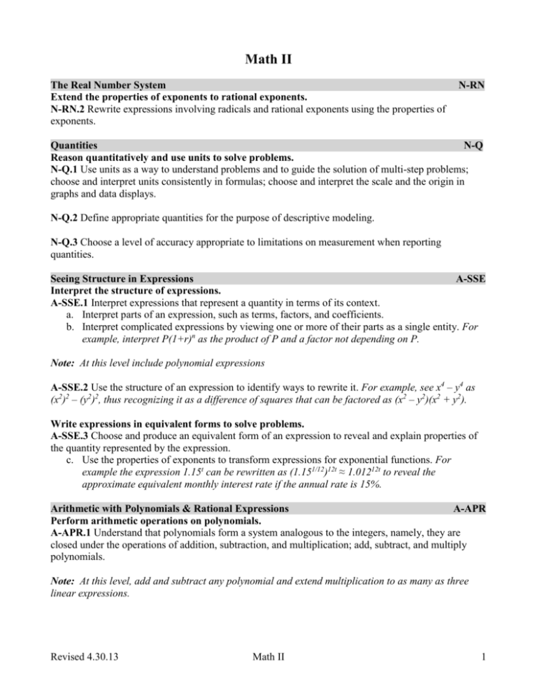
Math II
The Real Number System
Extend the properties of exponents to rational exponents.
N-RN.2 Rewrite expressions involving radicals and rational exponents using the properties of
exponents.
N-RN
Quantities
N-Q
Reason quantitatively and use units to solve problems.
N-Q.1 Use units as a way to understand problems and to guide the solution of multi-step problems;
choose and interpret units consistently in formulas; choose and interpret the scale and the origin in
graphs and data displays.
N-Q.2 Define appropriate quantities for the purpose of descriptive modeling.
N-Q.3 Choose a level of accuracy appropriate to limitations on measurement when reporting
quantities.
Seeing Structure in Expressions
A-SSE
Interpret the structure of expressions.
A-SSE.1 Interpret expressions that represent a quantity in terms of its context.
a. Interpret parts of an expression, such as terms, factors, and coefficients.
b. Interpret complicated expressions by viewing one or more of their parts as a single entity. For
example, interpret P(1+r)n as the product of P and a factor not depending on P.
Note: At this level include polynomial expressions
A-SSE.2 Use the structure of an expression to identify ways to rewrite it. For example, see x4 – y4 as
(x2)2 – (y2)2, thus recognizing it as a difference of squares that can be factored as (x2 – y2)(x2 + y2).
Write expressions in equivalent forms to solve problems.
A-SSE.3 Choose and produce an equivalent form of an expression to reveal and explain properties of
the quantity represented by the expression.
c. Use the properties of exponents to transform expressions for exponential functions. For
example the expression 1.15t can be rewritten as (1.151/12)12t ≈ 1.01212t to reveal the
approximate equivalent monthly interest rate if the annual rate is 15%.
Arithmetic with Polynomials & Rational Expressions
A-APR
Perform arithmetic operations on polynomials.
A-APR.1 Understand that polynomials form a system analogous to the integers, namely, they are
closed under the operations of addition, subtraction, and multiplication; add, subtract, and multiply
polynomials.
Note: At this level, add and subtract any polynomial and extend multiplication to as many as three
linear expressions.
Revised 4.30.13
Math II
1
Understand the relationship between zeros and factors of polynomials.
A-APR.3 Identify zeros of polynomials when suitable factorizations are available, and use the zeros to
construct a rough graph of the function defined by the polynomial.
Note: At this level, limit to quadratic expressions.
Creating Equations
A-CED
Create equations that describe numbers or relationships.
A-CED.1 Create equations and inequalities in one variable and use them to solve problems. Include
equations arising from linear and quadratic functions, and simple rational and exponential functions.
Note: At this level extend to quadratic and inverse variation (the simplest rational) functions and use
common logs to solve exponential equations.
A-CED.2 Create equations in two or more variables to represent relationships between quantities;
graph equations on coordinate axes with labels and scales.
Note: At this level extend to simple trigonometric equations that involve right triangle trigonometry.
A-CED.3 Represent constraints by equations or inequalities, and by systems of equations and/or
inequalities, and interpret solutions as viable or nonviable options in a modeling context. For example,
represent inequalities describing nutritional and cost constraints on combinations of different foods.
Note: Extend to linear-quadratic, and linear–inverse variation (simplest rational) systems of
equations.
A-CED.4 Rearrange formulas to highlight a quantity of interest, using the same reasoning as in solving
equations. For example, rearrange Ohm’s law V = IR to highlight resistance R.
Note: At this level, extend to compound variation relationships.
Reasoning with Equations & Inequalities
A-REI
Understand solving equations as a process of reasoning and explain the reasoning.
A-REI.1 Explain each step in solving a simple equation as following from the equality of numbers
asserted at the previous step, starting from the assumption that the original equation has a solution.
Construct a viable argument to justify a solution method.
Note: At this level, limit to factorable quadratics.
A-REI.2 Solve simple rational and radical equations in one variable, and give examples showing how
extraneous solutions may arise.
Note: At this level, limit to inverse variation.
Revised 4.30.13
Math II
2
Solve equations and inequalities in one variable.
A-REI.4 Solve quadratic equations in one variable.
b. Solve quadratic equations by inspection (e.g., for x2 = 49), taking square roots, completing
the square, the quadratic formula and factoring, as appropriate to the initial form of the
equation. Recognize when the quadratic formula gives complex solutions and write them as a ±
bi for real numbers a and b.
Note: At this level, limit solving quadratic equations by inspection, taking square roots, quadratic
formula, and factoring when lead coefficient is one. Writing complex solutions is not expected;
however recognizing when the formula generates non-real solutions is expected.
Solve systems of equations.
A-REI.7 Solve a simple system consisting of a linear equation and a quadratic equation in two
variables algebraically and graphically. For example, find the points of intersection between the line
y = –3x and the circle x2 + y2 = 3.
Represent and solve equations and inequalities graphically.
A-REI.10 Understand that the graph of an equation in two variables is the set of all its solutions
plotted in the coordinate plane, often forming a curve (which could be a line).
Note: At this level, extend to quadratics.
A-REI.11 Explain why the x-coordinates of the points where the graphs of the equations y = f(x) and
y = g(x) intersect are the solutions of the equation f(x) = g(x); find the solutions approximately, e.g.,
using technology to graph the functions, make tables of values, or find successive approximations.
Include cases where f(x) and/or g(x) are linear, polynomial, rational, absolute value, exponential, and
logarithmic functions.
Note: At this level, extend to quadratic functions.
Interpreting Functions
F-IF
Understand the concept of a function and use function notation.
F-IF.2 Use function notation, evaluate functions for inputs in their domains, and interpret statements
that use function notation in terms of a context.
Note: At this level, extend to quadratic, simple power, and inverse variation functions.
Interpret functions that arise in applications in terms of the context.
F-IF.4 For a function that models a relationship between two quantities, interpret key features of
graphs and tables in terms of the quantities, and sketch graphs showing key features given a verbal
description of the relationship. Key features include: intercepts; intervals where the function is
increasing, decreasing, positive, or negative; relative maximums and minimums; symmetries; end
behavior; and periodicity.
Note: At this level, limit to simple trigonometric functions (sine, cosine, and tangent in standard
position) with angle measures of 180° (𝜋 𝑟𝑎𝑑𝑖𝑎𝑛𝑠) or less. Periodicity not addressed.
Revised 4.30.13
Math II
3
F-IF.5 Relate the domain of a function to its graph and, where applicable, to the quantitative
relationship it describes. For example, if the function h(n) gives the number of person-hours it takes to
assemble n engines in a factory, then the positive integers would be an appropriate domain for the
function.
Note: At this level, extend to quadratic, right triangle trigonometry, and inverse variation functions.
Analyze functions using different representations.
F-IF.7 Graph functions expressed symbolically and show key features of the graph, by hand in simple
cases and using technology for more complicated cases.
b. Graph square root, cube root, and piecewise-defined functions, including step functions and
absolute value functions.
e. Graph exponential and logarithmic functions, showing intercepts and end behavior, and
trigonometric functions, showing period, midline, and amplitude.
Note: At this level, extend to simple trigonometric functions (sine, cosine, and tangent in standard
position)
F-IF.8 Write a function defined by an expression in different but equivalent forms to reveal and
explain different properties of the function.
a. Use the process of factoring and completing the square in a quadratic function to show zeros,
extreme values, and symmetry of the graph, and interpret these in terms of a context.
Note: At this level, completing the square is still not expected.
F-IF.9 Compare properties of two functions each represented in a different way (algebraically,
graphically, numerically in tables, or by verbal descriptions). For example, given a graph of one
quadratic function and an algebraic expression for another, say which has the larger maximum.
Note: At this level, extend to quadratic, simple power, and inverse variation functions.
Building Functions
F-BF
Build a function that models a relationship between two quantities.
F-BF.1 Write a function that describes a relationship between two quantities.
a. Determine an explicit expression, a recursive process, or steps for calculation from a context.
Note: Continue to allow informal recursive notation through this level.
b. Combine standard function types using arithmetic operations. For example, build a function
that models the temperature of a cooling body by adding a constant function to a decaying
exponential, and relate these functions to the model.
Build new functions from existing functions.
F-BF.3 Identify the effect on the graph of replacing f(x) by f(x) + k, k f(x), f(kx), and f(x + k) for
specific values of k (both positive and negative); find the value of k given the graphs. Experiment with
cases and illustrate an explanation of the effects on the graph using technology. Include recognizing
even and odd functions from their graphs and algebraic expressions for them.
Note: At this level, extend to quadratic functions and, k f(x).
Revised 4.30.13
Math II
4
Congruence
G-CO
Experiment with transformations in the plane
G-CO.2 Represent transformations in the plane using, e.g., transparencies and geometry software;
describe transformations as functions that take points in the plane as inputs and give other points as
outputs. Compare transformations that preserve distance and angle to those that do not (e.g., translation
versus horizontal stretch).
G-CO.3 Given a rectangle, parallelogram, trapezoid, or regular polygon, describe the rotations and
reflections that carry it onto itself.
G-CO.4 Develop definitions of rotations, reflections, and translations in terms of angles, circles,
perpendicular lines, parallel lines, and line segments.
G-CO.5 Given a geometric figure and a rotation, reflection, or translation, draw the transformed figure
using, e.g., graph paper, tracing paper, or geometry software. Specify a sequence of transformations
that will carry a given figure onto another.
Understand congruence in terms of rigid motions
G-CO.6 Use geometric descriptions of rigid motions to transform figures and to predict the effect of a
given rigid motion on a given figure; given two figures, use the definition of congruence in terms of
rigid motions to decide if they are congruent.
G-CO.7 Use the definition of congruence in terms of rigid motions to show that two triangles are
congruent if and only if corresponding pairs of sides and corresponding pairs of angles are congruent.
G-CO.8 Explain how the criteria for triangle congruence (ASA, SAS, and SSS) follow from the
definition of congruence in terms of rigid motions.
Prove geometric theorems
G-CO.10 Prove theorems about triangles. Theorems include: measures of interior angles of a triangle
sum to 180°; base angles of isosceles triangles are congruent; the segment joining midpoints of two
sides of a triangle is parallel to the third side and half the length; the medians of a triangle meet at a
point.
Note: At this level, include measures of interior angles of a triangle sum to 180° and the segment
joining midpoints of two sides of a triangle is parallel to the third side and half the length.
Make geometric constructions
G-CO.13 Construct an equilateral triangle, a square, and a regular hexagon inscribed in a circle.
Similarity, Right Triangles, & Trigonometry
G-SRT
Understand similarity in terms of similarity transformations
G-SRT.1 Verify experimentally the properties of dilations given by a center and a scale factor:
a. A dilation takes a line not passing through the center of the dilation to a parallel line, and leaves
a line passing through the center unchanged.
b. The dilation of a line segment is longer or shorter in the ratio given by the scale factor.
Revised 4.30.13
Math II
5
Define trigonometric ratios and solve problems involving right triangles
G-SRT.6 Understand that by similarity, side ratios in right triangles are properties of the angles in the
triangle, leading to definitions of trigonometric ratios for acute angles.
G-SRT.7 Explain and use the relationship between the sine and cosine of complementary angles.
G-SRT.8 Use trigonometric ratios and the Pythagorean Theorem to solve right triangles in applied
problems.
Apply trigonometry to general triangles
G-SRT.9 (+) Derive the formula A = 1/2 ab sin(C) for the area of a triangle by drawing an auxiliary
line from a vertex perpendicular to the opposite side.
G-SRT.11 (+) Understand and apply the Law of Sines and the Law of Cosines to find unknown
measurements in right and non-right triangles (e.g., surveying problems, resultant forces).
Expressing Geometric Properties with Equations
G-GPE
Translate between the geometric description and the equation for a conic section
G-GPE.1 Derive the equation of a circle of given center and radius using the Pythagorean Theorem;
complete the square to find the center and radius of a circle given by an equation.
Note: At this level, derive the equation of the circle using the Pythagorean Theorem.
G-GPE.6 Find the point on a directed line segment between two given points that partitions the
segment in a given ratio.
Geometric Measurement and Dimension
G-GMD
Visualize relationships between two-dimensional and three-dimensional objects
G-GMD.4 Identify the shapes of two-dimensional cross-sections of three-dimensional objects, and
identify three-dimensional objects generated by rotations of two-dimensional objects.
Modeling with Geometry
G-MG
Apply geometric concepts in modeling situations
G-MG.1 Use geometric shapes, their measures, and their properties to describe objects (e.g., modeling
a tree trunk or a human torso as a cylinder).
G-MG.2 Apply concepts of density based on area and volume in modeling situations (e.g., persons per
square mile, BTUs per cubic foot).
G-MG.3 Apply geometric methods to solve design problems (e.g., designing an object or structure to
satisfy physical constraints or minimize cost; working with typographic grid systems based on ratios).
Making Inferences & Justifying Conclusions
S-IC
Understand and evaluate random processes underlying statistical experiments
S-IC.2 Decide if a specified model is consistent with results from a given data-generating process, e.g.,
using simulation. For example, a model says a spinning coin falls heads up with probability 0.5. Would
a result of 5 tails in a row cause you to question the model?
Revised 4.30.13
Math II
6
Make inferences and justify conclusions from sample surveys, experiments, and observational
studies
S-IC.6 Evaluate reports based on data.
Conditional Probability and the Rules of Probability
S-CP
Understand independence and conditional probability and use them to interpret data
S-CP.1 Describe events as subsets of a sample space (the set of outcomes) using characteristics (or
categories) of the outcomes, or as unions, intersections, or complements of other events (“or,” “and,”
“not”).
S-CP.2 Understand that two events A and B are independent if the probability of A and B occurring
together is the product of their probabilities, and use this characterization to determine if they are
independent.
S-CP.3 Understand the conditional probability of A given B as P(A and B)/P(B), and interpret
independence of A and B as saying that the conditional probability of A given B is the same as the
probability of A, and the conditional probability of B given A is the same as the probability of B.
S-CP.4 Construct and interpret two-way frequency tables of data when two categories are associated
with each object being classified. Use the two-way table as a sample space to decide if events are
independent and to approximate conditional probabilities. For example, collect data from a random
sample of students in your school on their favorite subject among math, science, and English. Estimate
the probability that a randomly selected student from your school will favor science given that the
student is in tenth grade. Do the same for other subjects and compare the results.
S-CP.5 Recognize and explain the concepts of conditional probability and independence in everyday
language and everyday situations. For example, compare the chance of having lung cancer if you are a
smoker with the chance of being a smoker if you have lung cancer.
Use the rules of probability to compute probabilities of compound events in a uniform
probability model
S-CP.6 Find the conditional probability of A given B as the fraction of B’s outcomes that also belong
to A, and interpret the answer in terms of the model.
S-CP.7 Apply the Addition Rule, P(A or B) = P(A) + P(B) – P(A and B), and interpret the answer in
terms of the model.
S-CP.8 (+) Apply the general Multiplication Rule in a uniform probability model, P(A and B) =
P(A)P(B|A) = P(B)P(A|B), and interpret the answer in terms of the model.
S-CP.9 (+) Use permutations and combinations to compute probabilities of compound events and
solve problems.
Revised 4.30.13
Math II
7