Curvilinear Bivariate Regression
You are now familiar with linear bivariate regression analysis. What do you do if the
relationship between X and Y is curvilinear? It may be possible to get a good analysis with our usual
techniques if we first “straighten-up” the relationship with data transformations.
You may have a theory or model that indicates the nature of the nonlinear effect. For example,
if you had data relating the physical intensity of some stimulus to the psychologically perceived
intensity of the stimulus, Fechner’s law would suggest a logarithmic function (Stevens’ would suggest
a power function). To straighten out this log function all you would need to do is take the log of the
physical intensity scores and then complete the regression analysis using transformed physical
intensity scores to predict psychological intensity scores. For another example, suppose you have
monthly sales data for each of 25 consecutive months of a new business. You remember having
been taught about exponential growth curves in a business or a biology class, so you do the
regression analysis for predicting the log of monthly sales from the number of months the firm has
been in business.
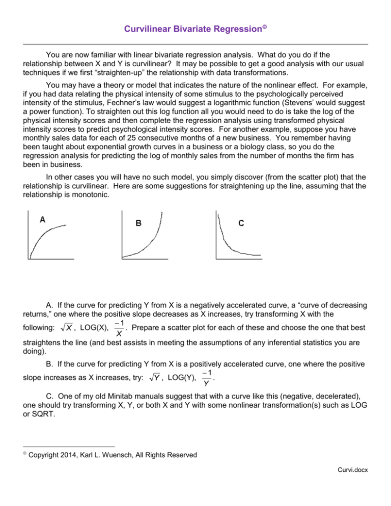
In other cases you will have no such model, you simply discover (from the scatter plot) that the
relationship is curvilinear. Here are some suggestions for straightening up the line, assuming that the
relationship is monotonic.
A. If the curve for predicting Y from X is a negatively accelerated curve, a “curve of decreasing
returns,” one where the positive slope decreases as X increases, try transforming X with the
1
following: X , LOG(X),
. Prepare a scatter plot for each of these and choose the one that best
X
straightens the line (and best assists in meeting the assumptions of any inferential statistics you are
doing).
B. If the curve for predicting Y from X is a positively accelerated curve, one where the positive
1
slope increases as X increases, try: Y , LOG(Y),
.
Y
C. One of my old Minitab manuals suggest that with a curve like this (negative, decelerated),
one should try transforming X, Y, or both X and Y with some nonlinear transformation(s) such as LOG
or SQRT.

Copyright 2014, Karl L. Wuensch, All Rights Reserved
Curvi.docx
You can always just try a variety of nonlinear transformations and see what works best. One
handy transformation is to RANK the data. When done on both variables, the resulting r is a
Spearman correlation coefficient.
To do a square root transformation of variable Y in SAS, use a statement like this in the data
step: X_Sqrt = SQRT(X); for a base ten log transformation, X_Log = LOG10(X); for an inverse
transformation, X_Inv = -1/X; . If you have scores of 0 or less, you will need to add an appropriate
constant (to avoid scores of 0 or less) to X before applying a square root or log transformation, for
example, X_Log = LOG10(X + 19); .
Please look at this example of the use of a log transformation where the relationship is
nonlinear, negative, monotonic.
Polynomial Regression
Monotonic nonlinear transformations (such as SQRT, LOG, and -1/X) of independent and/or
dependent variables may allow you to obtain a predictive model that has less error than does a linear
model, but if the relationship between X and Y is not monotonic, a polynomial regression may do a
better job. A polynomial has two or more terms. The polynomials we most often use in simple
polynomial regression are the quadratic, Yˆ  a  b1 X  b2 X 2 , and the cubic,
Yˆ  a  b X  b X 2  b X 3 . With a quadratic, the slope for predicting Y from X changes direction
1
2
3
once, with a cubic it changes direction twice.
Please run the program Curvi.sas from my SAS Programs page. This provides an example of
how to do a polynomial regression with SAS. The data were obtained from scatterplots in an article
by N. H. Copp (Animal Behavior, 31,: 424-430). Ladybugs tend to form large winter aggregations,
clinging to one another in large clumps, perhaps to stay warm. In the laboratory, Copp observed, at
various temperatures, how many beetles (in groups of 100) were free (not aggregated). For each
group tested, we have the temperature at which they were tested and the number of ladybugs that
were free. Note that in the data step I create the powers of the temperature variable (temp2, temp3,
and temp4).
Please note that a polynomial regression analysis is a sequential analysis. One first
evaluates a linear model. Then one adds a quadratic term and decides whether or not addition of
such a term is justified. Then one adds a cubic term and decides whether or not such an addition is
justified, etc.
Proc Reg is used to test linear, quadratic, cubic, and quartic models. The VAR statement is
used to list all of the variables that will be used in the models that are specified.
The LINEAR model replicates the analysis which Copp reported. Note that there is a strong (r2
= .615) and significant (t = 7.79, p < .001) linear relationship between temperature and number of free
ladybugs. Inspection of the residuals plots, however, shows that I should have included temperaturesquared in the model, making it a quadratic model. After contemplating how complex I am willing to
make the model, I decide to evaluate linear, quadratic, cubic, and quartic models.
I next evaluated the QUARTIC model, requesting Type I (sequential) sums of squares and
Type I squared semipartial correlation coefficients. From the output I can see that adding
temperature-squared to the linear model significantly increases the R2, and by a large amount, .223.
Adding temperature-cubed to the quadratic model significantly increases the R2, but by a small
amount, .023. I ponder whether that small increase in R2 justifies making the model more complex. I
end, somewhat reluctantly, keeping temperature-cubed in the model. Finally, I see that adding
2
temperature4 to the cubic model increased the R2 by a small and not significant amount, so I revert to
the cubic model
For pedagogical purposes, I created plots of the linear model, the quadratic model, and the
cubic model.
The plot for the quadratic model shows that aggregation of the ladybugs is greatest at about 5
to 10 degrees Celsius (the mid to upper 40’s Fahrenheit). When it gets warmer than that, the
ladybugs start dispersing, but they also start dispersing when it gets cooler than that. Perhaps
ladybugs are threatened by temperatures below freezing, so the dispersal at the coldest temperatures
represents their attempt to find a warmer place to aggregate.
The second bend in the curve provided by a cubic model is not very apparent in the plot of the
cubic model, but there is an apparent flattening of the line at low temperatures. It would be really
interesting to see what would happen if the ladybugs were tested at temperatures even lower than
those employed by Copp.
Below is an example of how to present results of a polynomial regression. I used SPSS to
produce the figure.
Forty groups of ladybugs (100 ladybugs per group) were tested at temperatures ranging
from -2 to 34 degrees Celsius. In each group I counted the number of ladybugs which were free (not
aggregated). A polynomial regression analysis was employed to fit the data with an appropriate
model. To be retained in the final model, a component had to be statistically significant at the .05
level and account for at least 2% of the variance in the number of free ladybugs. The model adopted
was a cubic model, Free Ladybugs = 13.607 + .085 Temperature - .022 Temperature2 + .001
Temperature3, F(3, 36) = 74.50, p < .001, η2 = .86, 90% CI [.77, .89]. Table 1 shows the contribution
of each component at the point where it entered the model. It should be noted that a quadratic model
fit the data nearly as well as did the cubic model.
Table 1.
Number of Free Ladybugs Related to Temperature
Component
SS
df
t
p
sr2
Linear
853
1
7.79
< .001
.61
Quadratic
310
1
7.15
< .001
.22
Cubic
32
1
2.43
.020
.02
As shown in Figure 1, the ladybugs were most aggregated at temperatures of 18 degrees or
less. As temperatures increased beyond 18 degrees, there was a rapid rise in the number of free
ladybugs.
3
Current research in my laboratory is directed towards evaluating the response of ladybugs
tested at temperatures lower than those employed in the currently reported research. It is anticipated
that the ladybugs will break free of aggregations as temperatures fall below freezing, since remaining
in such a cold location could kill a ladybug.
Polynomial Regression with I/O Data
Megan Waggy (2014) investigated the relationships between employee commitment and
demographic variables. One of the commitment variables was continuance commitment, the
employee’s ‘need’ to stay with the organization. The employee evaluates the costs associated with
leaving the organization and if the costs are too high, the employee feels unable to leave and is found
to have high levels of continuance commitment. The costs include the personal sacrifice associated
with leaving the organization, such as loss of salary, loss of friends, and loss of job progress. These
costs may be moderated by the availability of alternative employment.
Megan’s review of the literature revealed that studies of the relationship between
organizational commitment and tenure have been mixed – sometimes positive, sometimes negative,
sometimes trivial. It occurred to me that this might result from the relationship not being linear. My
4
thinking was that by mid-career an employee might have developed the skills and connection that
make em able to get alternative employment elsewhere and that as an employee approaches
retirement the need for continued employment will drop. A re-analysis of Megan’s data confirmed the
hypothesized nonlinear relationship.
We used SPSS to conduct the analysis.
Click Next and select Tenure squared (created with Transform, Compute). Then click Next
and add Tenure cubed.
5
Model
1
2
3
R
R
Square
.045a
.261b
.288c
Change Statistics
R Square
F
df1
df2
Change
Change
.002
.352
1
174
.066
12.241
1
173
.015
2.775
1
172
.002
.068
.083
Sig. F
Change
.554
.001
.098
Notice that adding tenure cubed increased the R2 by a small and insignificant amount.
Accordingly, we drop back to the quadratic model. Also notice that the strength of association is a
helluva lot lower than it was with ladybugs. Well, explaining the behavior of humans is a bit more
difficult than explaining the behavior of ladybugs. 
ANOVAa
Model
Sum of
Squares
Regression
df
Mean
Square
4.096
.649
6.308
.002c
3.325
5.173
.002d
.243
.691
120.283
174
2
Total
Regression
Residual
Total
Regression
120.526
8.192
112.334
120.526
9.975
175
2
173
175
3
Residual
110.551
172
Total
120.526
175
3
.554b
1
Residual
Sig.
.352
.243
1
F
.643
a. Dependent Variable: Cont_Comm
b. Predictors: (Constant), Tenure_Years
c. Predictors: (Constant), Tenure_Years, Tenure2
d. Predictors: (Constant), Tenure_Years, Tenure2, Tenure3
Presenting the Results
Sequential polynomial regression analysis was employed to investigate the nature of the
relationship between tenure and continuance commitment. After evaluating a linear model, each
additional step involved entering the next highest power of the predictor (tenure, in years). This
continued until the addition of the next highest power increased the fit of the model to the data by an
insignificant or otherwise trivial amount. As shown in Table 1, adding a quadratic component to the
model produced a significant increase in fit, but adding a cubic component did not. Accordingly, the
quadratic model was adopted, F(2, 173) = 6.308, p = .002, R2 = .068 (see Figure 1).
6
Table 1
Predicting Continuance Commitment from Years of Tenure
df
p
Step
R2
F for R2
1: Linear
.002
0.352
1, 174 .554
2: Quadratic .066
12.241
1, 173 .001
3: Cubic
.015
2.775
1, 172 .098
Figure 1
Relationship Between Tenure and Continuance Commitment
References
Waggy, M. R. (2014). Self-reported changes in organizational commitment: the relationship between
present organizational commitment and its perceived changes over time. Not yet published
masters thesis, East Carolina University.
Back to Wuensch’s Stats Lessons Page
The ladybugs data in an Excel spreadsheet

Copyright 2014, Karl L. Wuensch, All Rights Reserved
7