-20
-30
-40
-10
20
10
0
-10
The polynomial interpolation problem can be stated as the following:
𝐺𝑖𝑣𝑒𝑛 𝑛 + 1 𝑑𝑎𝑡𝑎 𝑝𝑜𝑖𝑛𝑡𝑠, (𝑥 𝑖
, 𝑦 𝑖
-) 𝑓𝑜𝑟 𝑖 = 0,1, … 𝑛 𝑓𝑖𝑛𝑑 𝑎 𝑝(𝑥) ∈ 𝒫 𝑛
𝑠𝑢𝑐ℎ 𝑡ℎ𝑎𝑡 𝑝(𝑥 𝑖
) = 𝑦 𝑖
𝑓𝑜𝑟 𝑎𝑙𝑙 𝑖 = 0,1, … 𝑛 𝑤ℎ𝑒𝑟𝑒 𝒫 𝑛
𝑑𝑒𝑛𝑜𝑡𝑒𝑠 𝑡ℎ𝑒 𝑠𝑒𝑡 𝑜𝑓 𝑎𝑙𝑙 𝑝𝑜𝑙𝑦𝑛𝑜𝑚𝑖𝑎𝑙𝑠 𝑜𝑓 𝑑𝑒𝑔𝑟𝑒𝑒 𝑎𝑡 𝑚𝑜𝑠𝑡 𝑛
Example
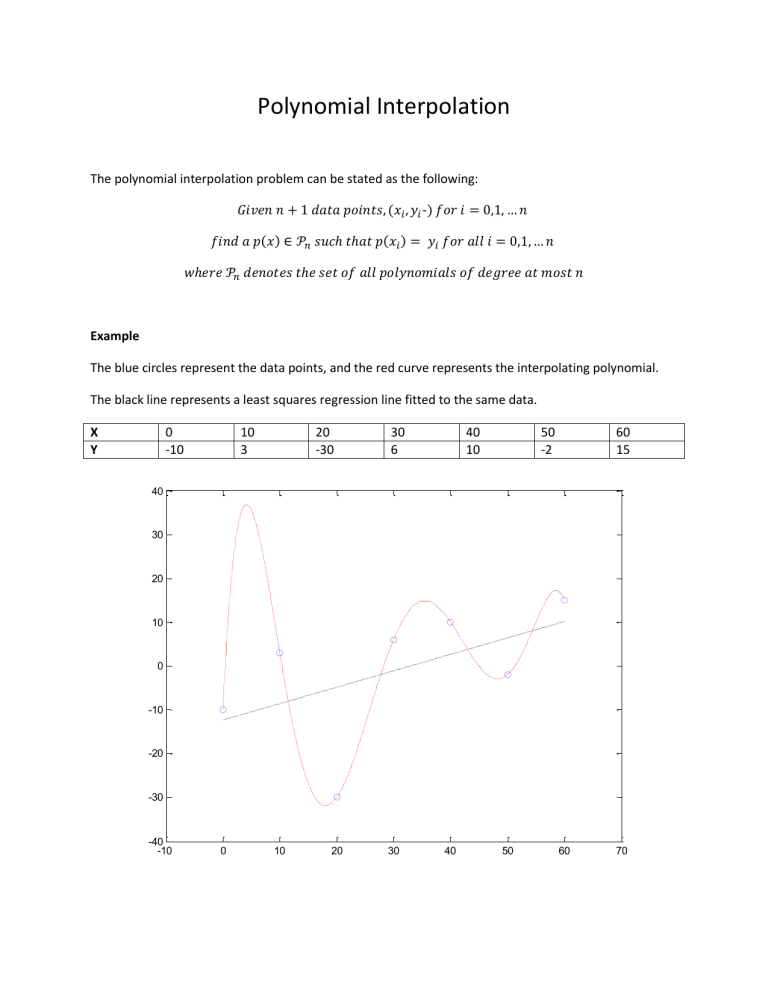
The blue circles represent the data points, and the red curve represents the interpolating polynomial.
The black line represents a least squares regression line fitted to the same data.
X
Y
0
-10
10
3
20
-30
30
6
40
10
50
-2
60
15
40
30
0 10 20 30 40 50 60 70

Interpolation vs. Regression
Interpolation models must take on the exact values of the known data points, whereas regression models try to minimize the distance between the prediction and each actual known value.
Given n+1 data points, the “best fit” polynomials of degree < n form regression models, where the predictions may not necessarily land exactly on the data points. However, the “best fit” polynomial of degree = n forms the interpolating polynomial which will land exactly on every data point. Notice that this means the sum of squared errors for the interpolating polynomial is always zero.
Interpolation vs. Regression Examples
-2
-3
-1
0
-1
3
2
1
-0.8
-0.6
-0.4
-0.2
0 0.2
0.4
0.6
0.8
1
1.5
1
-0.5
-1
-1.5
-1
0.5
0
-0.8
-0.6
-0.4
-0.2
0 0.2
0.4
0.6
0.8
1

Polynomial interpolation can be used when you believe your measured data to be exact.
Regression models, on the other hand, assume that measurements have noise. The model is usually: 𝑦 = 𝑓(𝑥) + 𝜀 𝑤ℎ𝑒𝑟𝑒 𝜀~𝑛(0, 𝜎 2 )
The point of a regression model is to estimate f(x), and this estimate can be used for forecasting future and past data values as well as predicting data values between known data points.
However, interpolation models are suitable only for estimating data values between data points.
Runge Phenomenon example
The function being sampled is:
1
1+16𝑥 2
The blue curve is f(x), the red curve is the interpolating polynomial, and the green curve is a spline
5 nodes 9 nodes
0.6
0.4
0.2
0
-0.2
-0.4
-0.6
-1
1.2
1
0.8
0.6
0.4
0.2
0
-0.2
-0.4
-0.6
-1
1.2
1
0.8
-0.8
-0.6
-0.4
-0.2
0 0.2
0.4
0.6
0.8
1
-0.6
-0.4
-0.8
17 nodes
-0.2
0 0.2
0.4
0.6
0.8
1
0.6
0.4
0.2
0
-0.2
-0.4
-0.6
-1
1.2
1
0.8
0.6
0.4
0.2
0
-0.2
-0.4
-0.6
-1
1.2
1
0.8
-0.8
-0.6
-0.4
-0.6
-0.8
21 nodes
-0.4
-0.2
-0.2
0 0.2
0.4
0.6
0.8
1
0 0.2
0.4
0.6
0.8
1

Solving the Polynomial Interpolation Problem
𝑈𝑠𝑖𝑛𝑔 {1, 𝑥, 𝑥 2 , 𝑥 3 , … 𝑥 𝑛 } 𝑎𝑠 𝑎 𝑏𝑎𝑠𝑖𝑠 𝑓𝑜𝑟 𝒫 𝑛 𝑎𝑛𝑦 𝑝(𝑥) ∈ 𝒫 𝑛
𝑐𝑎𝑛 𝑏𝑒 𝑤𝑟𝑖𝑡𝑡𝑒𝑛 𝑖𝑛 𝑡ℎ𝑒 𝑓𝑜𝑟𝑚: 𝑝(𝑥) = 𝛼
0
+ 𝛼
1 𝑥 + 𝛼
2 𝑥 2 + ⋯ + 𝛼 𝑛 𝑥 𝑛 𝑓𝑜𝑟 𝛼 𝑖
∈ ℝ
𝑂𝑢𝑟 𝑝𝑟𝑜𝑏𝑙𝑒𝑚 𝑏𝑒𝑐𝑜𝑚𝑒𝑠 𝑓𝑖𝑛𝑑𝑖𝑛𝑔 𝑡ℎ𝑒 𝛼 𝑖
𝑠𝑢𝑐ℎ 𝑡ℎ𝑎𝑡 𝑔𝑖𝑣𝑒𝑛 𝑛 + 1 𝑑𝑎𝑡𝑎 𝑝𝑜𝑖𝑛𝑡𝑠, (𝑥 𝑖
, 𝑦 𝑖
-) 𝑓𝑜𝑟 𝑖 = 0,1, … 𝑛 𝛼
0
+ 𝛼
1 𝑥 𝑖
+ 𝛼
2 𝑥 𝑖
2 + ⋯ + 𝛼 𝑛 𝑥 𝑖 𝑛 = 𝑦 𝑖
It is clear that this problem is simply a system of linear equations. We can set up the problem as
[
1 𝑥 0
1 𝑥
1 𝑥 𝑥
2
0
2
1
⋯
… 𝑥 𝑥
⋮ ⋮ ⋮ ⋱ ⋮ 𝑛
0 𝑛
1
1 𝑥 𝑛 𝑥 2 𝑛
… 𝑥 𝑛 𝑛
] [
𝛼 0 𝛼
⋮
1 𝛼 𝑛
]
=
[
𝑦 0 𝑦
⋮
1 𝑦 𝑛
]
We can use any normal solution method for solving systems of linear equations to find our solution.
The solution will be the interpolating polynomial 𝑝(𝑥) = 𝛼
0
+ 𝛼
1 𝑥 + 𝛼
2 𝑥 2 + ⋯ + 𝛼 𝑛 𝑥 𝑛

Matlab Implementation function result = poly_interp(x, y)
% x and y are column vectors with the x and y values of the data points
% there are n+1 data points n = length(x) - 1;
% construct the Vandermonde matrix
V = zeros(n+1,n+1); for i=1:n+1 for j=1:n+1
V(i,j) = x(i).^(j-1); end %for end %for
% solve the system of equations alpha = V\y;
%reverse the alpha vector to match Matlab standards
%for polynomial coefficient vectors result = fliplr(alpha');
% plot the solution xx = x(1):0.01:x(n+1); yp = polyval(result,xx); figure(100) plot(x,y, 'bo' ) hold on plot(xx,yp, 'r' ) end %function
Or you can just use the polyfit(x,y,n) function in Matlab. This function will find the polynomial of degree
n, which fits the data x and y best in a least squares sense. However, since the sum of squared errors for the interpolating polynomial is always zero, calling this function with n = #data points – 1 will give you the interpolating polynomial—instead of a regression polynomial—as a result.