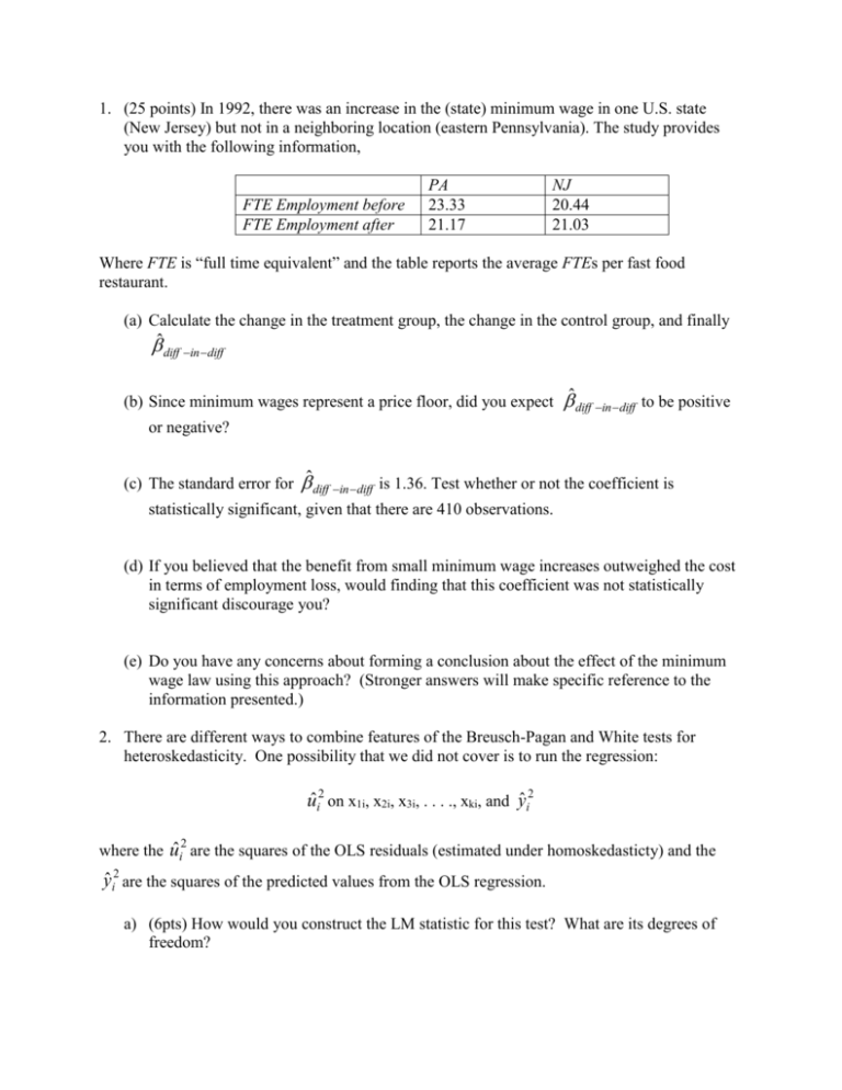
1. (25 points) In 1992, there was an increase in the (state) minimum wage in one U.S. state
(New Jersey) but not in a neighboring location (eastern Pennsylvania). The study provides
you with the following information,
FTE Employment before
FTE Employment after
PA
23.33
21.17
NJ
20.44
21.03
Where FTE is “full time equivalent” and the table reports the average FTEs per fast food
restaurant.
(a) Calculate the change in the treatment group, the change in the control group, and finally
̂ diff in diff
(b) Since minimum wages represent a price floor, did you expect
̂ diff in diff to be positive
or negative?
(c) The standard error for
̂ diff in diff is 1.36. Test whether or not the coefficient is
statistically significant, given that there are 410 observations.
(d) If you believed that the benefit from small minimum wage increases outweighed the cost
in terms of employment loss, would finding that this coefficient was not statistically
significant discourage you?
(e) Do you have any concerns about forming a conclusion about the effect of the minimum
wage law using this approach? (Stronger answers will make specific reference to the
information presented.)
2. There are different ways to combine features of the Breusch-Pagan and White tests for
heteroskedasticity. One possibility that we did not cover is to run the regression:
uˆi2 on x1i, x2i, x3i, . . . ., xki, and yˆ i2
where the uˆi are the squares of the OLS residuals (estimated under homoskedasticty) and the
2
yˆ i2 are the squares of the predicted values from the OLS regression.
a) (6pts) How would you construct the LM statistic for this test? What are its degrees of
freedom?
b) (5pts) How will the R2 from this regression compare with the R2 from the usual BP test
and the White test?
c) (5pts) Does this imply that the new test statistic always delivers a smaller/larger p-value
than the BP or White tests? Explain.
d) (5pts) Suppose someone suggested also adding ŷi to this regression. What do you think
of this idea?
3. For a large university, you are asked to estimate the demand for tickets to women’s
basketball games. You can collect time series data over 10 seasons, for a total of about 150
observations (assuming about 15 games a season. One possible model is
lATTENDt= β0+ β1lPRICEt+ β2 WINPERCt +β3 RIVALt +β4WEEKENDt + ut
where lATTEND is the natural log of attendance at a game, lPRICE is the natural log of the real
price of admissions, WINPERC is the team’s winning percentage, RIVAL is a dummy variable
indicating whether the game is with the major rival, and WEEKEND is a dummy variable for
whether or not the game is on a weekend.
a.
Do you think a time trend should be included in the equation? Why or why not?
b.
The supply of tickets is fixed by stadium capacity which has not changed over this
time period. Does this mean that price is necessarily exogenous (uncorrelated with
ut) in the equation? Explain.
c.
Suppose that the nominal price of admission changes slowly—say at the beginning of
each season. The athletic office chooses the price based partly on last season’s
average attendance, as well as the last season’s team success. If lPRICEt is in fact
endogenous, under what assumptions is last season’s winning percentage a valid
instrument for lPRICEt?
[NOTE: YOU CAN SKIP THIS PART AS WE HAVEN”T DONE IV YET]
d.
Suppose you are worried that some of the series, particularly lATTEND and lPRICE
might have unit roots. Why would this be a concern? How might you change the
estimated equation if these series did in fact have unit roots?
e.
If some games are sold out, what problems does this cause for estimating the demand
function?
4. One type of partial adjustment model is
y*t = 0 + 1xt+et
yt-yt-1 = (y*t-yt-1) + ut
where y*t is the desired or optimal level of y and yt is the actual observed level. For example, y*t
is the desired growth in firm inventories and xt is growth in firm sales. The parameter 1
measures the effect of xt on y*t. The second equation describes how the actual y depends on the
relationship between the desired y in time t and the actual y in time t-1. The parameter 
measures the speed of adjustment and satisfies 0<<1.
a.
Show that we can rewrite the model as a regression of yt on xt and yt-1. Show how the
coefficients in this model relate to the parameters in the two equation model above,
and show how the error term relates to the error terms above.
b.
If E(et|xt, yt-1, xt-1, yt-2, . . . .) = E(ut|xt, yt-1, xt-1, yt-2, . . . .) = 0 and all series are weakly
dependent, if we estimate the model you specified in (a) by OLS will we get
consistent estimates? Explain why or why not.
c.
Will the errors in your model in (a) be serially correlated? Explain why or why not.
5. Let hy6t denote the three-month holding yield (in percent) from buying a 6 month T-bill at
time (t-1) and selling it at time t (three months later) as a three month T bill.Let hy3t-1 be the
three month holding yield (in percent) from buying a 3 month T bill at time (t-1). At time (t1), then, hy3t-1 is known, whereas hy6t is unknown because the price in time t of three month
T-bills is unknown at time t-1.
The expectations hypothesis says that, of course, these two different three month investments
should be the same, on average. In other words,
E(hy6t|all information up to time t-1) = hy3t-1
Suppose you were to estimate the model
hy6t = 0 + 1 hy3t-1 + ut
a. 4 pts How would you test the expectations hypothesis using this model? What is the null
hypothesis?
b. 4pts Suppose your estimates of that equation produced the following
^hy6t = -.058 + 1.104 hy3t-1 + ut
(.070) (.039)
N=123, R2 = .866
Do you reject the test in (a) at the 5% significance level?
c. 4pts Another implication of the expectations hypothesis is that no other variables dated as
t-1 or earlier should explain hy6t after controlling for hy3t-1. Suppose you were to test
this implication by estimating the following equation, which includes the lagged spread
between the 6 and 3 month T-bill rates:
^hy6t = -.123+ 1.053 hy3t-1 + .480(r6t-1 – r3t-1)
(.067) (.039)
(.109)
According to this, is the lagged spread term significant at the 5% level? What do the
results imply about whether you should invest in 6-month or 3-month T bills if at
time t-1, r6 is greater than r3?
d. 3pts Conduct the test you specified in (a) using the results in (c). Do you conclude
anything different from your results in (b)?
e. 6pts The sample correlation between hy3t and hy3t-1 is .914. Does this raise any concerns
with your previous analysis? Be specific.
6. Suppose an author has data on outcomes (Y) for two periods, 1 and 2, for a number of crosssectional units (e.g., firms). Suppose also that a subgroup of firms were hit with an
intervention (e.g., minimum wage hike) sometime between period 1 and 2.
(b) 6 pts Write an equation for the difference-in-difference estimate (e.g., one that
controls for group and time effects) that provides a consistent estimate of the
intervention by using the first differences in outcomes between two periods. That is,
the dependent variable would be ΔYi = Y2i-Y1i.
(c) 5 pts What is the advantage of the difference-in difference approach in this context?
(d) 5pts Are there potential problems with inference that the difference-in-difference
approach does not resolve?