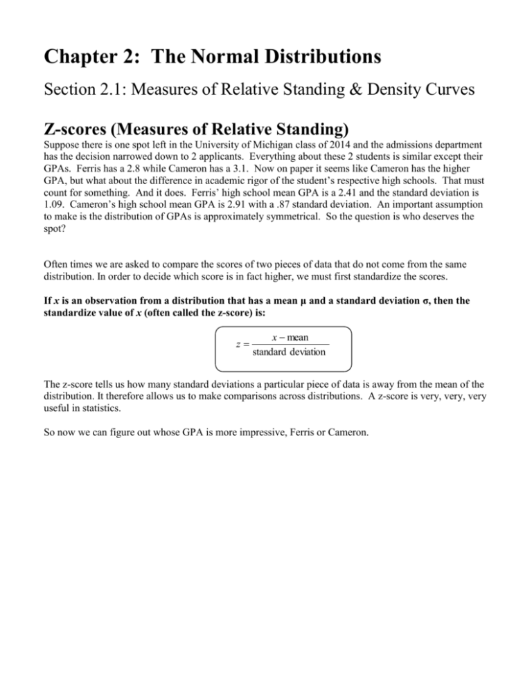
Chapter 2: The Normal Distributions
Section 2.1: Measures of Relative Standing & Density Curves
Z-scores (Measures of Relative Standing)
Suppose there is one spot left in the University of Michigan class of 2014 and the admissions department
has the decision narrowed down to 2 applicants. Everything about these 2 students is similar except their
GPAs. Ferris has a 2.8 while Cameron has a 3.1. Now on paper it seems like Cameron has the higher
GPA, but what about the difference in academic rigor of the student’s respective high schools. That must
count for something. And it does. Ferris’ high school mean GPA is a 2.41 and the standard deviation is
1.09. Cameron’s high school mean GPA is 2.91 with a .87 standard deviation. An important assumption
to make is the distribution of GPAs is approximately symmetrical. So the question is who deserves the
spot?
Often times we are asked to compare the scores of two pieces of data that do not come from the same
distribution. In order to decide which score is in fact higher, we must first standardize the scores.
If x is an observation from a distribution that has a mean μ and a standard deviation σ, then the
standardize value of x (often called the z-score) is:
z
x  mean
standard deviation
The z-score tells us how many standard deviations a particular piece of data is away from the mean of the
distribution. It therefore allows us to make comparisons across distributions. A z-score is very, very, very
useful in statistics.
So now we can figure out whose GPA is more impressive, Ferris or Cameron.
Percentile (Measuring Relative Standing)
If you are trying to find the percentile corresponding to a certain score x:
Percentile 
number of scores < x
100
total number of scores
Percentiles are used often when reporting academic scores such as SAT scores. Let’s say you get a 620
on the math portion of the SAT. It might also indicate that you are in the “78th percentile”. That means
that you scored better than 78% of all students taking that particular SAT.
A few miscellaneous facts:
Pk is the notation for the kth percentile
P25  Q1
P50  Q2  median
P75  Q3
Qn is the notation for the nth quartile
Example: Here are the scores of 25 students on the chapter 1 test in AP Calculus
79
81
80
77
73
74
93
78
80
75
67
73
77
83
86
90
79
85
83
89
84
82
77
72
83
The score that is bolded is Eli Manning’s score. How did Eli do relative to his classmates?
Question: Is there a simple way of converting a z-score to a percentile?
Answer: YES, but it depends on the shape of the distribution
For example, if on a test, if your grade was exactly the mean grade of the entire class, what would your zscore be?
So would you assume that if you got the exact average grade then you would be in the 50th percentile
right? Not necessarily. If the distribution is heavily skewed to the left would you really be in the 50th
percentile?
Chebyshev’s Inequality
In ANY distribution, the percent of observations falling within k standard deviations of the mean is at
1
least (100) (1 − 𝑘 2 )
Fill in the blank using Chebyshev’s Inequality for k = 1 through 5
𝟏
k
at least (𝟏𝟎𝟎) (𝟏 − 𝒌𝟐 )of observations fall within k standard deviations of mean
1
at least _________% of observations fall within 1 standard deviation of mean.
2
at least _________% of observations fall within 2 standard deviations of mean.
3
at least _________% of observations fall within 3 standard deviations of mean.
4
at least _________% of observations fall within 4 standard deviations of mean.
5
at least _________% of observations fall within 5 standard deviations of mean.
Foreshadowing comment:
Chebyshev’s inequality holds for ANY distribution. The second half of this chapter is titled Normal
Distributions. We will get a lot more specific with Chebyshev’s inequality when the distribution is
Normal. We will call that more specific “rule” the 68-95-99.7 Rule.
Density Curves
So far we have worked only with jagged histograms and stem plots to analyze data. As we begin to explore more
fully the many statistical calculations and analyses one can perform on data it will become clear that working with
smooth curves is much easier than jagged histograms. These smooth curves are called Density curves.
Characteristics of a density curve
 A density curve is a smooth curve that describes the overall pattern of a distribution by showing
what proportions of observations (not counts) fall into a range of values.
 Areas under a density curve represent proportions of observations
 The scale of a density curve is adjusted in such a way that the total area under the curve is always
equal to 1
 The density curve is always on or above the horizontal axis.
 The median of a density curve is the equal areas point.
 The mean of a density curve is the balance point (like a see-saw) if the curve was made of solid
material.
 The mean and the median are equal in a symmetric density curve.
 The mean and the median are not equal in a skewed density curve.
Section 2.2: Normal Distributions
A Particularly important class of density curves are normal distributions. A density curve that is normally
distributed has the following characteristics:
 Symmetric
 Single peak
 Bell shape
The mean of a density curve (including the normal curve) is denoted by μ (the Greek lowercase letter mu)
and the standard deviation is denoted by σ (the Greek lowercase letter sigma)
All Normal distributions have the same overall shape. Any differences can be explained by μ and σ.
Calculus connection:
On the normal curve, at a distance of σ on either side of the mean μ, are two points. These points are
called inflection points and they signify where the curve changes concavity. The normal curve changes
from concave up to concave down at these points. To find the inflection points, you would need to find
the second derivative of the function.
An unbelievable property that all normal curves have is that they follow the 68-95-99.7 rule
In a normal distribution with mean μ and standard deviation σ :
 68% of the observations fall within 1 standard deviation of the mean.
 95% of the observations fall within 2 standard deviations of the mean.
 99.7% of the observations fall within 3 standard deviations of the mean.
The Standard Normal Distribution
All normal distributions share many common properties. In fact, all Normal distributions are the same if
we measure in units of size σ about the mean μ as center. Changing these units requires us to standardize.
The standard Normal distribution is the Normal distribution N(0,1) with mean 0 and standard
deviation 1.
We can also figure out the percentile of each student once we know their z-scores. In order to do that, we
need to understand Table A
Examples:
1.) Find the area under the standard normal curve to the left of z = 1.15
2.) Find the proportion of observations from the standard normal curve that are less than 1.15
3.) Find the probability of randomly selecting an individual from a normal population whose z-score is
1.15 or less.
4.) What percent of z-scores are less than or equal to 1.15?
In the last part of this course, we will be given a sample
data set and we will have to determine if the sample chosen
comes from a normal population. We will learn how to
figure that out right here. There are 3 methods.
ASSESSING NORMALITY
Method 1: Construct a histogram, stem and leaf plot or box plot to determine if the shape is
approximately bell shaped with symmetry about the mean. This is fairly easy because if you load the data
into your calculator, you can check a histogram very quickly.
Method 2: Check the normal probability plot (on TI-83). This is an easy and quick way to check for
normality. You are shooting for a normal probability plot that has a linear trend to it.
Method 3: You can improve upon the accuracy of methods 1 and 2 by checking to see if the 68-95-99.7
rule applies (approximately) to the data. Find the mean, and standard deviation of the data. Find out if
approximately 68% of the data points are within 1 standard deviation of the mean, 95% are within 2
standard deviations, and approximately 99.7% are within 3 standard deviations. The last method is
cumbersome, so only use it as a back-up plan.
Example: The following are the heights of 50 of my former male students, randomly selected from my
classes. Are male student heights at DHS normally distributed?
68, 68, 73, 74, 75, 68, 68, 66, 70, 72, 69, 63, 68, 69, 68, 65, 68, 67, 69, 70, 71, 68, 66, 72, 69, 69, 70, 67,
64, 69, 70, 71, 68, 68, 67, 67, 69, 65, 68, 70, 69, 67, 66, 61, 68, 69, 69, 71, 72, 70
Method 1:
Since the histogram looks approximately bell shaped and the boxplot looks somewhat symmetric, we can
say the data comes from a normal distribution.
Method 2:
Since the normal probability plot looks approximately linear, we can say the data comes from a normal
distribution.
Note: The line that is drawn, does not appear on the TI-83.
Method 3:
x  1s  68.56  2.59  (65.97,71.15)
Percent of data falling in this interval: ____________
x  2s  68.56  5.18  (63.38,73.74)
Percent of data falling in this interval: _____________
x  3s  68.56  7.77  (60.79,76.33)
Percent of data falling in this interval: ____________
Since the above percentages approximately fit the 68-95-99.7 rule, we can say the data comes from an
approximately normal distribution.