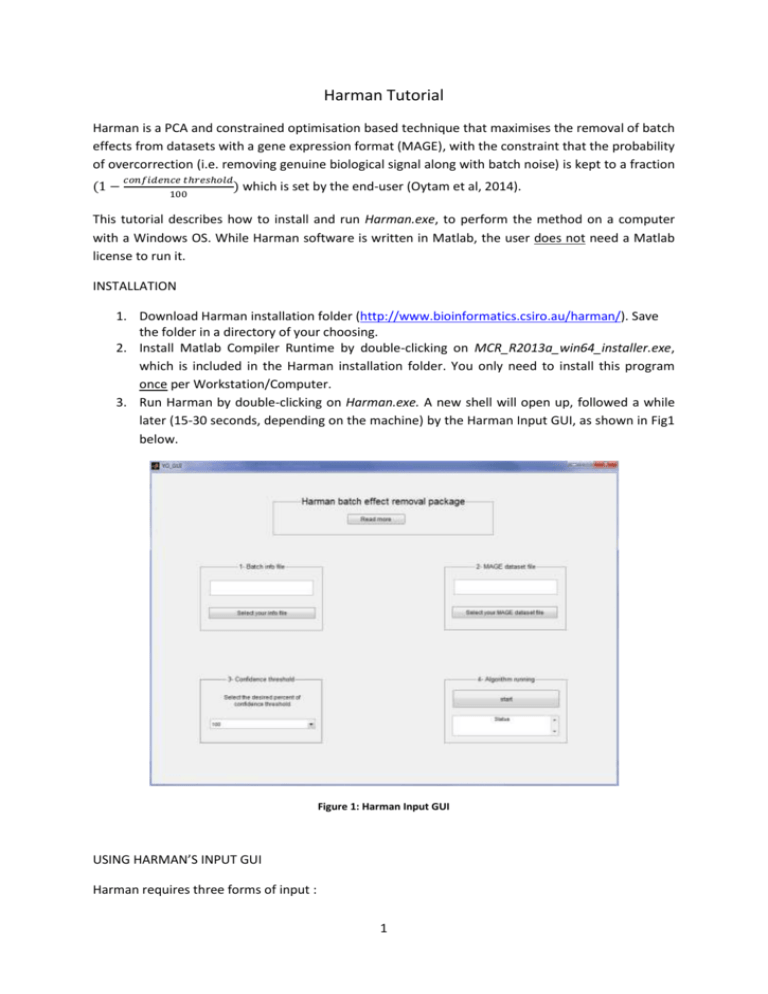
Harman Tutorial
Harman is a PCA and constrained optimisation based technique that maximises the removal of batch
effects from datasets with a gene expression format (MAGE), with the constraint that the probability
of overcorrection (i.e. removing genuine biological signal along with batch noise) is kept to a fraction
(1 −
𝑐𝑜𝑛𝑓𝑖𝑑𝑒𝑛𝑐𝑒 𝑡ℎ𝑟𝑒𝑠ℎ𝑜𝑙𝑑
) which
100
is set by the end-user (Oytam et al, 2014).
This tutorial describes how to install and run Harman.exe, to perform the method on a computer
with a Windows OS. While Harman software is written in Matlab, the user does not need a Matlab
license to run it.
INSTALLATION
1. Download Harman installation folder (http://www.bioinformatics.csiro.au/harman/). Save
the folder in a directory of your choosing.
2. Install Matlab Compiler Runtime by double-clicking on MCR_R2013a_win64_installer.exe,
which is included in the Harman installation folder. You only need to install this program
once per Workstation/Computer.
3. Run Harman by double-clicking on Harman.exe. A new shell will open up, followed a while
later (15-30 seconds, depending on the machine) by the Harman Input GUI, as shown in Fig1
below.
Figure 1: Harman Input GUI
USING HARMAN’S INPUT GUI
Harman requires three forms of input :
1
a. An ‘information file’ which describes the distribution of samples into 1-) batches,
and 2-) treatments/conditions,
b. A data file containing the dataset in gene expression format to be ‘cleansed’ of batch
effects,
c. A confidence threshold (%), limiting the probability of over-correction, and
essentially dictating the trade-off between signal preservation and noise rejection.
Figure 2: Two example files
The information file (.xlsx) consists of three columns. This first column includes the sample labels
from the data file. The second column specifies to which treatment the samples belong. The
treatments are numbered 1,2,...n, for n treatments. The third column specifies to which batch the
sample belongs. The batches are numbered 1,2,... m, for m batches, as shown in fig.3.
Figure 3: Sample info file
The data file is a matrix (also .xlsx) with expression values as rows and samples as columns, with
headers as depicted in fig.4. The first column consists of expression labels (Probeset IDs, or gene
symbols etc.), and the first row, of sample labels. The “sample label” in the information and data files
should match.
2
Figure 4: Sample data files
To select the information file, please hit the “Select your info file” button on the GUI which will open
up a new pop-up window, labelled “Select File to Open” (fig.5). Select your file and click “Open”. The
selected file will appear in the Harman GUI (fig.6).
Figure 3: Info file selection
3
Figure 4: Info file selected
To select the data file, please hit the “Select your MAGE dataset file” button on the GUI, which will
open up a new pop-up window, labelled “Select File to Open” (fig.7). Select your data file and click
“Open”. The selected file will appear in the Harman GUI (fig.8).
Figure 5: Data file selection
4
Figure 6: Data file selected
Next, select your confidence threshold by clicking the down arrow in the third box of the GUI. A popup menu will appear, displaying percentage scores, as shown in fig.9. Choosing 95%, for example,
will mean that potential batch effects will be removed from the data insofar as their probability of
arising out of empirical treatment distributions is less than 5% (i.e. 1-95%)
5
Figure 7: Selecting the confidence threshold
Now, press the start button to run the algorithm. A message will also appear in the “status” display
of the GUI (4th box) warning you that the progress bar may take some time to appear, depending on
the size and complexity of the dataset, and the processing capacity of your computer. A progress bar
will then appear, as shown in Figure 10.
6
Figure 8: Running the algorithm
VISUALISATION GUI
Once the algorithm is finished, a green coloured prompt will appear in the “status bar” informing
you that the process is complete. A new visualisation GUI will then appear (as shown in fig.11) with
two interactive PC plots displaying samples before and after batch correction. Any two PCs can be
selected in the “control panel” to be plotted. The effect of batch correction can be explored from the
PC plots. For the example dataset, the two highest corrections correspond to two smallest correction
numbers, 0.25 and 0.33, which belongs to PC1 and PC2 respectively, as displayed in fig.11.One
dimensional plots are also possible, by choosing the same PC for x and y axes (fig.12). The GUI will
also display the “correction vector”, indicating the (index of) PCs for which there was batch
correction and how much. The closer the displayed fraction to zero, the more the correction. The
user can click on the correction vector and scroll up and down the PC index by using the left and
right arrow keys on the keyboard, if necessary. PCs that are not listed in the “correction vector” are
not modified in any way – the algorithm would have found no batch effects for the confidence
threshold set by the user.
HARMAN’S OUTPUT FILES
Upon completion, Harman generates 3 new files and stores them in the same directory as the
original datafile: 1-) the corrected datafile in the original MAGE format, named originaldatafilenameHarmancorrectedXX.xlsx, where XX is the percentage confidence threshold chosen (for example, 95),
2-) the correction vector, named originaldatafilename-correctionvectorXX.xlsx and 3-) a matrix
consisting of the raw and corrected PC scores corresponding to the dataset, named
7
originaldatafilename-PCrawcorrXX.xlsx, with the matrix being [ PCraw PCcorrected], with column
vectors being the PCs and raw vectors being the samples.
Figure 9: PC visualization GUI
8
Figure 12: Using the GUI to show one-dimensional PC plots
DEMONSTRATION / EXAMPLE FILES
Data and information files are also included as examples in the Harman package, to get the user
started. They can be found in the “Example Files for Demonstration” folder. These consist of the
three datasets used in the Harman manuscript by Oytam et al.(2014), and the original data are from
Osmond et al (2013a), Osmond et al.(2013b), and Johnson et al. (2007).
REFERENCES
Johnson WE, Li C, Rabinovic A. 2007. Adjusting batch effects in microarray data using empirical bayes
methods. Biostatistics 8: 118–127.
Osmond-McLeod MJ, Osmond RIW, Oytam Y, McCall MJ, Feltis B, Mackay-Sim A, Wood SA, Cook AL.
2013a. Surface coatings of ZnO nanoparticles mitigate differentially a host of transcriptional, protein
and signalling responses in primary human olfactory cells. Particle and Fibre Toxicology. 10:54.
Osmond-McLeod MJ, Oytam Y, Kirby JK, Gomez-Fernandez L, Baxter B, McCall MJ. 2013b. Dermal
absorption and short-term biological impact in hairless mice from sunscreens containing zinc oxide
nano- or larger particles . Nanotoxicology, Early on-line, 1-13.
9
Oytam Y, Sobhanmanesh F, Ross J, Osmond-McLeod MJ, Duesing K (2014). Risk-conscious correction
of batch effects: Maximising information extraction from high-throughput genomic datasets (under
review)
10