A Brief Introduction to Reliability, Validity, and Scaling
Reliability
Simply put, a reliable measuring instrument is one which gives you the same
measurements when you repeatedly measure the same unchanged objects or events.
We shall briefly discuss here methods of estimating an instrument’s reliability. The
theory underlying this discussion is that which is sometimes called “classical
measurement theory.” The foundations for this theory were developed by Charles
Spearman (1904, “General Intelligence,” objectively determined and measures.
American Journal of Psychology, 15, 201-293).
If a measuring instrument were perfectly reliable, then it would have a perfect
positive (r = +1) correlation with the true scores. If you measured an object or event
twice, and the true scores did not change, then you would get the same measurement
both times.
We theorize that our measurements contain random error, but that the mean
error is zero. That is, some of our measurements have error that make them lower than
the true scores, but others have errors that make them higher than the true scores, with
the sum of the score-decreasing errors being equal to the sum of the score increasing
errors. Accordingly, random error will not affect the mean of the measurements, but it
will increase the variance of the measurements.
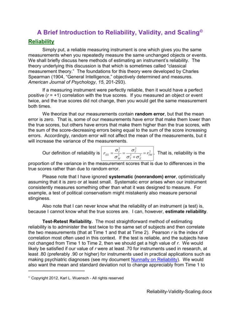
Our definition of reliability is rXX 
 T2
 T2
2

 rTM
. That is, reliability is the
 M2  T2   E2
proportion of the variance in the measurement scores that is due to differences in the
true scores rather than due to random error.
Please note that I have ignored systematic (nonrandom) error, optimistically
assuming that it is zero or at least small. Systematic error arises when our instrument
consistently measures something other than what it was designed to measure. For
example, a test of political conservatism might mistakenly also measure personal
stinginess.
Also note that I can never know what the reliability of an instrument (a test) is,
because I cannot know what the true scores are. I can, however, estimate reliability.
Test-Retest Reliability. The most straightforward method of estimating
reliability is to administer the test twice to the same set of subjects and then correlate
the two measurements (that at Time 1 and that at Time 2). Pearson r is the index of
correlation most often used in this context. If the test is reliable, and the subjects have
not changed from Time 1 to Time 2, then we should get a high value of r. We would
likely be satisfied if our value of r were at least .70 for instruments used in research, at
least .80 (preferably .90 or higher) for instruments used in practical applications such as
making psychiatric diagnoses (see my document Nunnally on Reliability). We would
also want the mean and standard deviation not to change appreciably from Time 1 to

Copyright 2012, Karl L. Wuensch - All rights reserved
Reliability-Validity-Scaling.docx
2
Time 2. On some tests, however, we would expect some increase in the mean due to
practice effects.
Alternate/Parallel Forms Reliability. If there two or more forms of a test, we
want to know that the two forms are equivalent (on means, standard deviations, and
correlations with other measures) and highly correlated. The r between alternate forms
can be used as an estimate of the tests’ reliability.
Split-Half Reliability. It may be prohibitively expensive or inconvenient to
administer a test twice to estimate its reliability. Also, practice effects or other changes
between Time 1 and Time 2 might invalidate test-retest estimates of reliability. An
alternative approach is to correlate scores on one random half of the items on the test
with the scores on the other random half. That is, just divide the items up into two
groups, compute each subject’s score on the each half, and correlate the two sets of
scores. This is like computing an alternate forms estimate of reliability after producing
two alternate forms (split-halves) from a single test. We shall call this coefficient the
half-test reliability coefficient, rhh.
Spearman-Brown. One problem with the split-half reliability coefficient is that it
is based on alternate forms that have only one-half the number of items that the full test
has. Reducing the number of items on a test generally reduces it reliability coefficient.
To get a better estimate of the reliability of the full test, we apply the Spearman-Brown
2rhh
correction, rsb 
.
1  rhh
Cronbach’s Coefficient Alpha. Another problem with the split-half method is
that the reliability estimate obtained using one pair of random halves of the items is
likely to differ from that obtained using another pair of random halves of the items.
Which random half is the one we should use? One solution to this problem is to
compute the Spearman-Brown corrected split-half reliability coefficient for every one of
the possible split-halves and then find the mean of those coefficients. This mean is
known as Cronbach’s coefficient alpha. Instructions for computing it can be found in my
document Cronbach’s Alpha and Maximized Lambda4.
Maximized Lambda4. H. G. Osburn (Coefficient alpha and related internal
consistency reliability coefficients, Psychological Methods, 2000, 5, 343-355) noted that
coefficient alpha is a lower bound to the true reliability of a measuring instrument, and
that it may seriously underestimate the true reliability. They used Monte Carlo
techniques to study a variety of alternative methods of estimating reliability from internal
consistency. Their conclusion was that maximized lambda4 was the most consistently
accurate of the techniques.
4 is the rsb for one pair of split-halves of the instrument. To obtain maximized 4,
one simply computes 4 for all possible split-halves and then selects the largest
.5(2n)!
obtained value of 4. The problem is that the number of possible split halves is
(n! ) 2
for a test with 2n items. If there are only four or five items, this is tedious but not
3
unreasonably difficult. If there are more than four or five items, computing maximized 4
is unreasonably difficulty, but it can be estimated -- see my document Estimating
Maximized Lambda4.
Construct Validity
Simply put, the construct validity of an operationalization (a measurement or a
manipulation) is the extent to which it really measures (or manipulates) what it claims to
measure (or manipulate). When the dimension being measured is an abstract construct
that is inferred from directly observable events, then we may speak of
“construct validity.”
Face Validity. An operationalization has face validity when others agree that it
looks like it does measure or manipulate the construct of interest. For example, if I tell
you that I am manipulating my subjects’ sexual arousal by having them drink a pint of
isotonic saline solution, you would probably be skeptical. On the other hand, if I told
you I was measuring my male subjects’ sexual arousal by measuring erection of their
penises, you would probably think that measurement to have face validity.
Content Validity. Assume that we can detail the entire population of behavior
(or other things) that an operationalization is supposed to capture. Now consider our
operationalization to be a sample taken from that population. Our operationalization will
have content validity to the extent that the sample is representative of the population.
To measure content validity we can do our best to describe the population of interest
and then ask experts (people who should know about the construct of interest) to judge
how well representative our sample is of that population.
Criterion-Related Validity. Here we test the validity of our operationalization by
seeing how it is related to other variables. Suppose that we have developed a test of
statistics ability. We might employ the following types of criterion-related validity:

Concurrent Validity. Are scores on our instrument strongly correlated with
scores on other concurrent variables (variables that are measured at the same
time). For our example, we should be able to show that students who just
finished a stats course score higher than those who have never taken a stats
course. Also, we should be able to show a strong correlation between score on
our test and students’ current level of performance in a stats class.

Predictive Validity. Can our instrument predict future performance on an
activity that is related to the construct we are measuring? For our example, is
there a strong correlation between scores on our test and subsequent
performance of employees in an occupation that requires the use of statistics.

Convergent Validity. Is our instrument well correlated with measures of other
constructs to which it should, theoretically, be related? For our example, we
might expect scores on our test to be well correlated with tests of logical thinking,
abstract reasoning, verbal ability, and, to a lesser extent, mathematical ability.

Discriminant Validity. Is our instrument not well correlated with measures of
other constructs to which it should not be related? For example, we might expect
4
scores on our test not to be well correlated with tests of political conservatism,
ethical ideology, love of Italian food, and so on.
Scaling
Scaling involves the construction of instruments for the purpose of measuring
abstract concepts such as intelligence, hypomania, ethical ideology, misanthropy,
political conservatism, and so on. I shall restrict my discussion to Likert scales, my
favorite type of response scale for survey items.
The items on a Likert scale consist of statements with which the respondents are
expected to differ with respect to the extent to which they agree with them. For each
statement the response scale may have from 4 to 9 response options. Because I have
used 5-point optical scanning response forms in my research, I have most often used
this response scale:
A
B
C
D
E
strongly disagree
disagree
no opinion
agree
strongly agree
Generating Potential Items. You should start by defining the concept you wish
to measure and then generate a large number of potential items. It is a good idea to
recruit colleagues to help you generating the items. Some of the items should be
worded such that agreement with them represents being high in the measured attribute
and others should be worded such that agreement with them represents being low in
the measured attribute.
Evaluating the Potential Items.
It is a good idea to get judges to evaluate your pool of potential items. Ask each
judge to evaluate each item using the following scale:
1 = agreeing indicates the respondent is very low in the measured attribute
2 = agreeing indicates the respondent is below average in the measured attribute
3 = agreeing does not tell anything about the respondent’s level of the attribute
4 = agreeing indicates the respondent is above average in the measured attribute
5 = agreeing indicates the respondent is very high in the measured attribute
Analyze the data from the judges and select items with very low or very high averages
(to get items with good discriminating ability) and little variability (indicating agreement
among the judges).
Alternatively, you could ask half of the judges to answer the items as they think a
person low in the attribute to be measured would, and the other half to answer the items
as would a person high in the attribute to be measured. You would then prefer items
which best discriminated between these two groups of judges -- items for which the
standardized difference between the group means is greatest.
5
Judges can also be asked whether any of the items were unclear or confusing or
had other problems.
Pilot Testing the Items. After you have selected what the judges thought were
the best items, you can administer the scale to respondents who are asked to answer
the questions in a way that reflects their own attitudes. It is a good idea to do this first
as a pilot study, but if you are impatient like me you can just go ahead and use the
instrument in the research for which you developed it (and hope that no really serious
flaws in the instrument appear). Even at this point you can continue your evaluation of
the instrument -- at the very least, you should conduct an item analysis (discussed
below), which might lead you to drop some of the items on the scale.
Scoring the Items. The most common method of creating a total score from a
set of Likert items is simply to sum each person’s responses to each item, where the
responses are numerically coded with 1 representing the response associated with the
lowest amount of the measured attribute and N (where N = the number of response
options) representing the response associated with the highest amount of the measured
attribute. For example, for the response scale I showed above, A = 1, B = 2, C = 3,
D = 4, and E = 5, assuming that the item is one for which agreement indicates having a
high amount of the measured attribute.
You need to be very careful when using a computer to compute total scores.
With some software, when you command the program to compute the sum of a certain
set of variables (responses to individual items), it will treat missing data (items on which
the respondent indicated no answer) as zeros, which can greatly corrupt your data. If
you have any missing data, you should check to see if this is a problem with the
computer software you are using. If so, you need to find a way to deal with that problem
(there are several ways, consult a statistical programmer if necessary).
I generally use means rather than sums when scoring Likert scales. This allows
me a simple way to handle missing data. I use the SAS (a very powerful statistical
analysis program) function NMISS to determine, for each respondent, how many of the
items are unanswered. Then I have the computer drop the data from any subject who
has missing data on more than some specified number of items (for example, more than
1 out of 10 items). Then I define the total score as being the mean of the items which
were answered. This is equivalent to replacing a missing data point with the mean of
the subject’s responses on the other items in that scale -- if all of the items on the scale
are measuring the same attribute, then this is a reasonable procedure. This can also be
easily done with SPSS.
If you have some items for which agreement indicates a low amount of the
measured attribute and disagreement indicates a high amount of the measured attribute
(and you should have some such items), you must remember to reflect (reverse score)
the item prior to including it in a total score sum or mean or an item analysis. For
example, consider the following two items from a scale that I constructed to measure
attitudes about animal rights:
 Animals should be granted the same rights as humans.
 Hunters play an important role in regulating the size of deer populations.
6
Agreement with the first statement indicates support for animal rights, but agreement
with the second statement indicates nonsupport for animal rights. Using the 5-point
response scale shown above, I would reflect scores on the second item by subtracting
each respondent’s score from 6.
Item Analysis. If you believe your scale is unidimensional, you will want to
conduct an item analysis. Such an analysis will estimate the reliability of your
instrument by measuring the internal consistency of the items, the extent to which the
items correlate well with one another. It will also help you identify troublesome items.
To illustrate item analysis with SPSS, we shall conduct an item analysis on data
from one of my past research projects. For each of 154 respondents we have scores
on each of ten Likert items. The scale is intended to measure ethical idealism. People
high on idealism believe that an action is unethical if it produces any bad
consequences, regardless of how many good consequences it might also produce.
People low on idealism believe that an action may be ethical if its good consequences
outweigh its bad consequences.
Bring the data (KJ-Idealism.sav) into SPSS.
Click Analyze, Scale, Reliability Analysis.
7
Select all ten items and scoot them to the Items box on the right.
Click the Statistics box.
Check “Scale if item deleted” and then click Continue.
Back on the initial window, click OK.
Look at the output. The Cronbach alpha is .744, which is acceptable.
8
Reliability Statistics
Cronbach's
Alpha
.744
N of Items
10
Look at the Item-Total Statistics.
Item-Total Statistics
Q1
Q2
Q3
Q4
Q5
Q6
Q7
Q8
Q9
Q10
Scale Mean if
Item Deleted
32.42
32.79
32.79
32.33
32.33
32.07
34.29
32.49
33.38
33.43
Scale
Variance if
Item Deleted
23.453
22.702
21.122
22.436
22.277
24.807
24.152
24.332
22.063
24.650
Corrected
Item-Total
Correlation
.444
.441
.604
.532
.623
.337
.247
.308
.406
.201
Cronbach's
Alpha if Item
Deleted
.718
.717
.690
.705
.695
.733
.749
.736
.725
.755
There are two items, numbers 7 and 10, which have rather low item-total
correlations, and the alpha would go up if they were deleted, but not much, so I retained
them. It is disturbing that item 7 did not perform better, since failure to do ethical
cost/benefit analysis is an important part of the concept of ethical idealism. Perhaps the
problem is that this item does not make it clear that we are talking about ethical
cost/benefit analysis rather than other cost/benefit analysis. For example, a person
might think it just fine to do a personal, financial cost/benefit analysis to decide whether
to lease a car or buy a car, but immoral to weigh morally good consequences against
morally bad consequences when deciding whether it is proper to keep horses for
entertainment purposes (riding them). Somehow I need to find the time to do some
more work on improving measurement of the ethical cost/benefit component of ethical
idealism.
1.
2.
3.
4.
5.
People should make certain that their actions never intentionally harm others
even to a small degree.
Risks to another should never be tolerated, irrespective of how small the risks
might be.
The existence of potential harm to others is always wrong, irrespective of the
benefits to be gained.
One should never psychologically or physically harm another person.
One should not perform an action which might in any way threaten the dignity
and welfare of another individual.
9
6.
7.
8.
9.
10.
If an action could harm an innocent other, then it should not be done.
Deciding whether or not to perform an act by balancing the positive
consequences of the act against the negative consequences of the act is
immoral.
The dignity and welfare of people should be the most important concern in any
society.
It is never necessary to sacrifice the welfare of others.
Moral actions are those which closely match ideals of the most "perfect" action.
Factor Analysis. It may also be useful to conduct a factor analysis on the scale
data to see if the scale really is unidimensional. Responses to the individual scale items
are the variables in such a factor analysis. These variables are generally well
correlated with one another. We wish to reduce the (large) number of variables to a
smaller number of factors that capture most of the variance in the observed variables.
Each factor is estimated as being a linear (weighted) combination of the observed
variables. We could extract as many factors as there are variables, but generally most
of those factors would contribute little, so we try to get just a few factors that capture
most of the covariance. Our initial extraction generally includes the restriction that the
factors be orthogonal, independent of one another.
Copyright 2012, Karl L. Wuensch - All rights reserved.
Return to Wuensch’s Statistics Lessons