RANDOM VARIABLES ISSUES WITH MEANS AND STANDARD DEVIATIONS
         
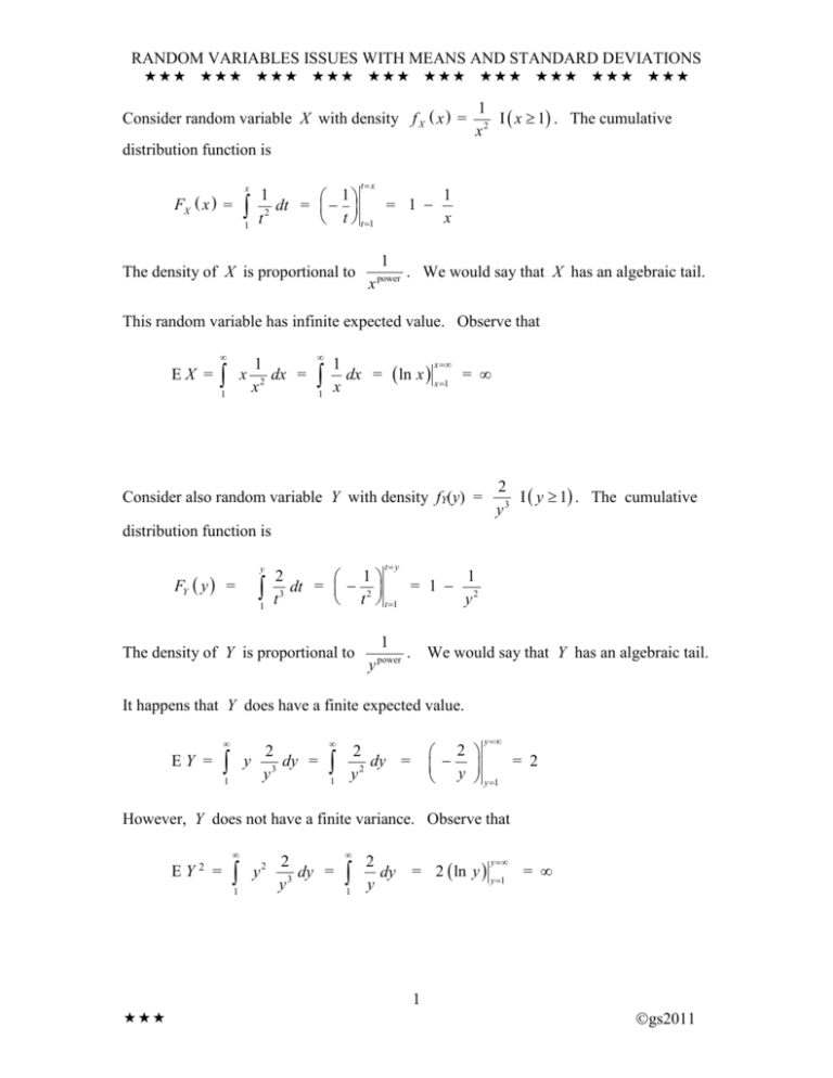
Consider random variable X with density f X  x  =
1
I  x  1 . The cumulative
x2
distribution function is
x
FX  x  =

1
tx
1
1
 1
= 1 
dt =   
2
x
t
 t  t 1
The density of X is proportional to
1
x
power
. We would say that X has an algebraic tail.
This random variable has infinite expected value. Observe that

EX =

x
1
1
dx =
x2


1
1
dx =
x
x 
 ln x  x 1
= ∞
Consider also random variable Y with density fY(y) =
2
I  y  1 . The cumulative
y3
distribution function is
FY  y  =
y

1
t y
1
2
 1
= 1  2
dt =   2 
3
y
t
 t  t 1
The density of Y is proportional to
1
y
power
.
We would say that Y has an algebraic tail.
It happens that Y does have a finite expected value.

2
y 3 dy =
y

EY =
1


1
y 
 2 
= 2
  y 

 y 1
2
dy =
y2
However, Y does not have a finite variance. Observe that

EY
2
=

1
y
2
2
dy =
y3


1
y 
2
dy = 2  ln y  y 1 = ∞
y
1

gs2011
RANDOM VARIABLES ISSUES WITH MEANS AND STANDARD DEVIATIONS
         
The random variable Q with density fQ  q  =
1
1
is centered at . It’s

 1   q   2
clear that  is the median. This is an example of the Cauchy distribution. The
cumulative distribution function is
FQ  q 
 u  tan 

= 

2
 du  sec  d 
1
=

q 
 u  t  
1
1
=  
dt = 
2

 1   t  
 du  dt 

q
tan 1  q  


d =

2
tan 1  q  



2


1
1

du
 1  u2
1
1

sec 2  d 
2
 1  tan 
1
1
1

1

tan 1  q  
 tan  q     =
2


2
The density of Q is proportional to
1
q
power
. We would say that Q has an algebraic tail.
It happens that Q is more pathological that the X and Y examples above. Only
positive values were possible for X and Y, so that their moments must be either finite
positive numbers or infinite. For Q, here’s what happens when we try to find the
mean:

EQ =



=


u
q
 u  q  
1
1

dq = 
2

 1   q  
 du  dq 
1
1

du 
 1  u2






 u   1  1 2 du
 1 u
u
1
1

du  
 1  u2


1
1

du =
 1  u2


The  part is no problem. As for the integral,



1
1
u 
du =
 1  u2
0


1
1
u 
du 
 1  u2

u
0
1
1

du
 1  u2
The first part is -∞ and the second is ∞. We will say for this random variable that “the
mean does not exist.” It would not be proper to say that the mean is infinite.
2

gs2011
RANDOM VARIABLES ISSUES WITH MEANS AND STANDARD DEVIATIONS
         
2
1

I  r  0  and
 1  r2
it will indeed have E R = ∞. Its behavior will be similar to that of X (page 1).
The “absolute Cauchy,” call it R, has density f R  r  =
We have more friendly random variables, however. The normal random variable W
with mean  and variance 2 has density
fW  w  =
1
 2  w  
1
e 2
 2
2
power
This density is proportional to e w
and has all its moments. For the normal, the
power in the exponent is 2, so the tails are really tight.
The exponential random variable V with mean  has density
1  v 
fV  v  =
e
I v  0

power
also has a density proportional to e v . The power in the exponent is 1, so the tails of
the exponential are not as tight as for the normal.
This raises interesting questions as to what large samples from these probability laws
would look like. If X1, X2, X3, X4, … is a sample from the density of X, it’s interesting
X  X 2  ...  X n
to look at the running average sequence { Xn }, where Xn = 1
. We’ll
n
X 
also examine the running Z-scores { Z nX }, where Z nX = n n
. These are

the computations we would make if we believed that the Central Limit theorem holds;
we’d do the math with whatever values  and  we believe are appropriate.
3

gs2011
RANDOM VARIABLES ISSUES WITH MEANS AND STANDARD DEVIATIONS
         
Suppose that we took a sample of 10,000 values from a normal population with mean
 = 200 and standard deviation  = 30. Here’s a plot of the running average:
Running Average from normal (mean 200, stdev 30)
210
200
190
RunAve
180
170
160
150
140
130
120
1
1000
2000
3000
4000
5000 6000
Index
7000
8000
9000
10000
This bumps around at the beginning. The first value was about 125. The running
average converges quickly to the mean 200, exactly as the law of large numbers (law of
averages) dictates.
Here is a plot of the running Z-scores:
Running Z-scores based on normal sample (mean 200, stdev 30)
2
Z-score
1
0
-1
-2
-3
1
1000
2000
3000
4000
5000
Index
6000
7000
8000
9000
10000
Typical Z-scores are between -2 and +2, so this looks quite reasonable.
4

gs2011
RANDOM VARIABLES ISSUES WITH MEANS AND STANDARD DEVIATIONS
         
The random variable X (from page 1) has an infinite mean. Here’s plot of the running
average:
Running Average from 1/(x*x)
22.5
20.0
RunAve
17.5
15.0
12.5
10.0
7.5
5.0
1
1000
2000
3000
4000
5000 6000
Index
7000
8000
9000
10000
This running average will drift away to +∞, although this happens in fits and starts.
Suppose that we thought that the mean was 10 and the standard deviation was 50. We’d
X n  10
compute the Z-scores as Z nX = n
. Here’s what that plot of those running
50
Z-scores would look like:
Running Z-scores from 1/(x*x)
12
Z-score
9
6
3
0
1
1000
2000
3000
4000
5000
Index
6000
7000
8000
9000
10000
Check the vertical scale! If the sample average is escaping to +∞, it’s going to be hard to
have a credible Z-score.
These two pictures have a crude similarity. But note that the first, based on Xn , is scaled
as 1n , while the second is scaled as 1n .
5

gs2011
RANDOM VARIABLES ISSUES WITH MEANS AND STANDARD DEVIATIONS
         
The random variable Y (page 1) has a finite mean but an infinite variance.
Running average from density 1/(x*x*x)
5
RunAve
4
3
2
1
1
1000
2000
3000
4000
5000
Index
6000
7000
8000
9000
10000
Here is a plot of the running Z-scores, using  = 2 (correct) and  = 2 (an irrelevant
guess, since the standard deviation is infinite):
Running Z-scores from 1/(x*x*x)
6
5
Z-score
4
3
2
1
0
-1
1
1000
2000
3000
4000
5000
Index
6000
7000
8000
9000
10000
Xn  
certainly

n
1
X 

has mean 0. The variance is Var  n n
 = 2 Var  X n    = 2 Var  X 1  .
 



Notice that this is X1. Since Var(X1) = ∞, this is infinite, but it’s not running wild very
quickly.
This looks erratic, but it’s not running amok. The random variable
6

n
gs2011
RANDOM VARIABLES ISSUES WITH MEANS AND STANDARD DEVIATIONS
         
Here is a plot of the running variance:
Running sample variances from density 1/(x*x*x)
120
Sample variance
100
80
60
40
20
0
1
1000
2000
3000
4000
5000 6000
Index
7000
8000
9000
10000
The variance of this random variable is infinite, and the sample variance will tend to
infinity. This plot suggests that it’s in no hurry to get there!
Why the slow march to infinity? The random variable X has infinite mean. The random
variable Y has finite mean but infinite variance.
Recall that

EX =
1
x 2 dx =
x

1

EY
2
=

1
y
2


1
2
dy =
y3

The story is that the integral

1
1,000,000
1
dx =
x
1
about 27.63.

1
dx =
x
x 1,000,000
 ln x  x1


1
x 
 ln x  x 1
y 
2
dy = 2  ln y  y 1 = ∞
y
1
dx explodes in a very, very slow style. Consider that
x
= ln(1,000,000)  13.82. The integral to 1012 is only
7

= ∞
gs2011
RANDOM VARIABLES ISSUES WITH MEANS AND STANDARD DEVIATIONS
         
So what does a sample from the Cauchy distribution look like? Consider the density
1
1
f(x) =
. Here’s a plot of the running average from a simulated sample

 1   x  50 2
of 10,000:
Running Average from Cauchy, centered at 50
Running Average
50
49
48
47
46
1
1000
2000
3000
4000
5000
Index
6000
7000
8000
9000
10000
The mean does not exist for this distribution, so the running average will move aimlessly.
The running variance is tending to infinity, but not in a regular fashion:
Running variance, Cauchy centered at 50
4000
Variance
3000
2000
1000
0
1
1000
2000
3000
4000
5000 6000
Index
8

7000
8000
9000 10000
gs2011