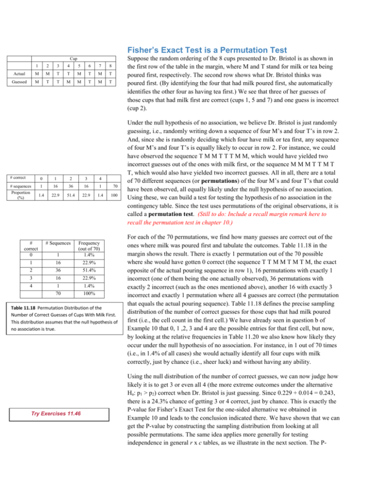
Fisher’s Exact Test is a Permutation Test
Suppose the random ordering of the 8 cups presented to Dr. Bristol is as shown in
the first row of the table in the margin, where M and T stand for milk or tea being
poured first, respectively. The second row shows what Dr. Bristol thinks was
poured first. (By identifying the four that had milk poured first, she automatically
identifies the other four as having tea first.) We see that three of her guesses of
those cups that had milk first are correct (cups 1, 5 and 7) and one guess is incorrect
(cup 2).
Cup
1
2
3
4
5
6
7
8
Actual
M
M
T
T
M
T
M
T
Guessed
M
T
T
M
M
T
M
T
# correct
0
1
2
3
4
# sequences
Proportion
(%)
1
16
36
16
1
70
1.4
22.9
51.4
22.9
1.4
100
#
correct
0
# Sequences
1
Frequency
(out of 70)
1.4%
1
16
22.9%
2
36
51.4%
3
16
22.9%
4
1
1.4%
70
100%
Table 11.18 Permutation Distribution of the
Number of Correct Guesses of Cups With Milk First.
This distribution assumes that the null hypothesis of
no association is true.
Try Exercises 11.46
Under the null hypothesis of no association, we believe Dr. Bristol is just randomly
guessing, i.e., randomly writing down a sequence of four M’s and four T’s in row 2.
And, since she is randomly deciding which four have milk or tea first, any sequence
of four M’s and four T’s is equally likely to occur in row 2. For instance, we could
have observed the sequence T M M T T T M M, which would have yielded two
incorrect guesses out of the ones with milk first, or the sequence M M M T T M T
T, which would also have yielded two incorrect guesses. All in all, there are a total
of 70 different sequences (or permutations) of the four M’s and four T’s that could
have been observed, all equally likely under the null hypothesis of no association.
Using these, we can build a test for testing the hypothesis of no association in the
contingency table. Since the test uses permutations of the original observations, it is
called a permutation test. (Still to do: Include a recall margin remark here to
recall the permutation test in chapter 10.)
For each of the 70 permutations, we find how many guesses are correct out of the
ones where milk was poured first and tabulate the outcomes. Table 11.18 in the
margin shows the result. There is exactly 1 permutation out of the 70 possible
where she would have gotten 0 correct (the sequence T T M M T M T M, the exact
opposite of the actual pouring sequence in row 1), 16 permutations with exactly 1
incorrect (one of them being the one actually observed), 36 permutations with
exactly 2 incorrect (such as the ones mentioned above), another 16 with exactly 3
incorrect and exactly 1 permutation where all 4 guesses are correct (the permutation
that equals the actual pouring sequence). Table 11.18 defines the precise sampling
distribution of the number of correct guesses for those cups that had milk poured
first (i.e., the cell count in the first cell.) We have already seen in question b of
Example 10 that 0, 1 ,2, 3 and 4 are the possible entries for that first cell, but now,
by looking at the relative frequencies in Table 11.20 we also know how likely they
occur under the null hypothesis of no association. For instance, in 1 out of 70 times
(i.e., in 1.4% of all cases) she would actually identify all four cups with milk
correctly, just by chance (i.e., sheer luck) and without having any ability.
Using the null distribution of the number of correct guesses, we can now judge how
likely it is to get 3 or even all 4 (the more extreme outcomes under the alternative
Ha: p1 > p2) correct when Dr. Bristol is just guessing. Since 0.229 + 0.014 = 0.243,
there is a 24.3% chance of getting 3 or 4 correct, just by chance. This is exactly the
P-value for Fisher’s Exact Test for the one-sided alternative we obtained in
Example 10 and leads to the conclusion indicated there. We have shown that we can
get the P-value by constructing the sampling distribution from looking at all
possible permutations. The same idea applies more generally for testing
independence in general r x c tables, as we illustrate in the next section. The P-
value is called an exact P-value because it uses the exact, not approximate,
sampling distribution.
Permutation Test for Independence or Homogeneity in
General r x c Tables
Recall From Section 11.2, X2 is a summary
measure of the differences between observed
and expected (under independence) cell
counts. The larger X2, the stronger the
evidence for an association.
Recall The chi-squared distribution is only
appropriate to use when all expected cell
counts are larger than 5. See Section 11.2.
The same procedure of a permutation test can be extended to general r x c tables.
The only difference to the 2 x 2 case is that we no longer can use the first cell (the
number of correctly identified cups with milk added first) as a test statistic, but need
a more general measure for the association. We will use one that we have used all
along to test for an association, the chi-squared statistic X2. However, finding the Pvalue under the chi-squared distribution with df = (r-1)(c-1) may no longer be
appropriate, because of small cell counts. Instead, we will find its permutation
distribution which will let us judge if the observed value of X2 is large or not. The
following example illustrates.
Example 12: Edward Snowden – Hero or
Criminal? (Use Tag: Permutation Test)
Picture the Scenario
In 2013, Edward Snowden revealed classified material about massive spying
activities by the U.S National Security Agency, not only on U.S citizens, but on
citizens worldwide. While the U.S. wants to try him in court for breaking several
laws, many other countries point out that the activities of the NSA severely violated
their privacy laws. In these countries, Snowden is often celebrated as a h. In a 2014
survey at Williams College, 12 U.S. students and 8 international students were
asked whether Edward Snowden should be considered a hero, a criminal, or neither.
Table 11.19 shows the results, for which X2 = 6.9. We want to test whether these
data provide evidence that the opinion on Edward Snowden differs between U.S.
and international students at Williams College. The null hypothesis is that the
conditional distributions are the same, i.e., homogeneity.
Table 11.19 Results from a survey conducted at Williams College on whether Edward
Snowden should be considered a hero, a criminal or neither. X2 = 6.9 for this table.
Student Status
U.S.
International
Total
Opinion on Edward Snowden
Hero
Criminal
Neither
1
9
2
5
2
1
6
11
3
Total
12
8
20
Question to Explore
a. Can we use the chi-squared distribution with df=(2-1)(3-1)=2 to find the P-value
for X2 = 6.9?
b. How can we construct the permutation distribution of X2 under the null
hypothesis of homogeneity?
Student
Status
Response
1
2
3
4
5
6
7
8
9
10
11
12
13
14
15
16
17
18
19
20
Int
US
US
US
US
US
US
US
US
Int
Int
US
Int
Int
Int
US
Int
Int
US
US
Hero
Criminal
Neither
Criminal
Hero
Criminal
Criminal
Criminal
Criminal
Criminal
Hero
Neither
Hero
Hero
Hero
Criminal
Criminal
Neither
Criminal
Criminal
Permutation
of Status
Labels
US
Int
US
Int
US
US
Int
US
US
Int
US
US
US
Int
US
US
Int
US
Int
Int
Caption: Original observations for data
summarized in Table 11.19. The last row
shows one permutation of the original status
labels.
c. How can we judge whether the observed value of 6.9 is extreme and find the
permutation P-value?
Think it Through
a. Many counts in Table 11.19 are small, leading to expected values that are
smaller than 5. For instance, the expected count is 3.6 in the first cell and 1.2 in the
last cell. Using the chi-squared distribution may lead to questionable conclusions
since it may not approximate the actual sampling distribution well.
b. The first three columns of the table in the margin show the raw data from the
survey, before summarizing it in Table 11.19. (You can check that there are, for
instance, 5 international students with response “Hero”.) Under the null hypothesis
of homogeneity, any given response is equally likely to have come from a U.S.
student or an international student. For instance, the probability of a student
selecting “Hero” does not depend on whether he is from the U.S or international.
Then, the status of a student is merely a label that loses its relevance under the null
hypothesis. We get a dataset that is equally likely to occur (under the null
hypothesis) when we permute these labels. This is similar to the tea tasting
experiment, where under the null hypothesis any permutation of the four M’s and
four T’s was equally likely to occur. Here, any permutation (or shuffling) of the
status labels for the 12 U.S. and 8 international students yields a dataset that is
equally likely to occur. The last column in the margin table shows one possible
permutation (out of a total of 125,970) of the 12 “US” and 8 “Int” labels. Taken
together with the response column, it leads to the cell counts shown in Table 11.20.
For instance, with the permuted status labels we now have only 1 international
student with response “Hero”.
Table 11.20 Contingency table based on the permuted status labels. X2 = 5.9 for this table.
Student
U.S.
International
Total
Opinion on Edward Snowden
Hero
Criminal
Neither
5
4
3
1
7
0
6
11
3
Total
12
8
20
Table 11.20 has the same row and column margins as the originally observed Table
11.19. (For any permutation, we will still have a total of 12 US and 8 international
students, as well as a total of 6 students responding “hero”, 11 students responding
“Criminal” and 2 students responding “Neither”.) However, the cell counts in the
body of the table differ from the ones in Table 11.19 and yield a chi-squared
statistic of X2 = 5.9.
A different permutation of the status labels results yet in another table with the
same margins but different cell counts. For each table resulting from a permutation
of the status labels we compute the chi-squared statistic X2. Note that several
permutations can give rise to the same table and hence X2 statistic. For instance, just
switching the last two labels for students 19 and 20 (both US students with response
“Criminal”) results in the same table (and hence X2 statistic) as the one observed.
X2
Freq.
(%)
0.3
#
Permutat
ions
20,790
16.5
Cumulat
ive Freq.
(%)
16.5
0.4
19,800
15.7
32.2
1.1
14,850
11.8
44.0
1.9
9,900
7.9
51.9
2.4
25,872
20.5
72.4
…
…
…
…
5.9
3,960
3.1
95.9
6.6
990
0.8
96.7
6.9
2,090
1.7
98.4
…
…
…
…
16.5
6
<0.0
100
17.2
3
<0.0
100
125,970
100%
100%
Caption: Excerpt of permutation
(=sampling) distribution of X2 based on
data in Table 11.19. For instance, 9,900
of all 125,970 permutations resulted in
X2 = 1.9 or 4,167 (=3.3%) of all
permutations result in an X2 as large or
larger than 6.9.
In Practice
When there are too many possible
permutations, one simply takes a
large random sample (such as
10,000) of them and computes
X2for each. The proportion among
them with X2 as large or larger is
then a very good approximation of
the actual permutation P-value.
Tabulating all the different values for X2 and how often they arise yields the
permutation distribution for X2. This is the sampling distribution of X2 under the
null hypothesis. We show an excerpt of it in the margin, while Figure 11.7 shows it
graphically.
Figure 11.7 Permutation distribution of X2 based on data in Table 11.19. The
black dot indicates the observed vale of X2= 6.9. Question: For tables with larger
cell counts than Table 11.19, the shape of the permutation distribution is
approximately equal to the shape of which distribution?
c. How extreme is the observed chi-squared statistic of 6.9? Figure 11.7 already
gives us an idea. The observed value is indicated by the black dot and seems to be
in the tail of the distribution. To find the permutation P-value, we need to find the
proportion of the 125,970 permutations that yielded a chi-squared statistic as large
or larger than the observed one. All in all, there are 4,167 permutations that yielded
a value for X2 as large or larger than 6.9, for a proportion of 4,167/125,970 =
0.0331. This is the permutation P-value for the chi-squared test. It indicates that
there is evidence that the opinion on Edward Snowden differs among U.S. and
international students.
Insight
The permutation approach is valid for any sample size, not just for small cell
counts. However, for larger tables and/or large sample sizes it quickly becomes
impossible to compute X2 for all possible permutations because there are just too
many. In these cases, one simply generates a large number of random permutations
and computes the proportion with an X2 value as large or larger than the one
observed. This provides a very accurate approximation of the permutation P-value.
We may choose this approach even for Table 11.19 above: Randomly generating
10,000 permutations by “shuffling” the status labels 10,000 times yielded 329 tables
with an X2 as large or larger than the observed one of 6.9. (Again, note that many of
these random shuffles result in identical tables.) This gives an approximate
permutation P-value of 329/10000 = 0.0329, close to the actual permutation Pvalue.
Try Exercises 11.45
Still to do: The next Activity shows how you can perform the permutation test for
your own data online, using a web app that runs in your browser.