Lesson 24
NYS COMMON CORE MATHEMATICS CURRICULUM
M4
ALGEBRA I
Lesson 24: Modeling with Quadratic Functions
Student Outcomes

Students create a quadratic function from a data set based on a contextual situation, sketch its graph, and
interpret both the function and the graph in context. They answer questions and make predictions related to
the data, the quadratic function, and graph.
Lesson Notes
MP.1
MP.2
MP.4
&
MP.6
Throughout this lesson, students make sense of problems by analyzing the given information; make sense of the
quantities in the context, including the units involved; look for entry points to a solution; consider analogous problems;
create functions to model situations; use graphs to explain or validate their reasoning; monitor their own progress and
the reasonableness of their answers; and report their results accurately and with an appropriate level of precision.
In this lesson, students understand that it takes three points to determine a unique quadratic function. They use data
sets to write quadratic functions with and without context. For convenience, the points used in the following exercises
have known 𝑦-intercepts and can be modeled precisely by quadratic functions with rational coefficients; however,
teachers should remind students that in real life, data sets are unlikely to be able to be modeled with any function with
100% accuracy.
Classwork
Opening Exercise (10 minutes)
Scaffolding:
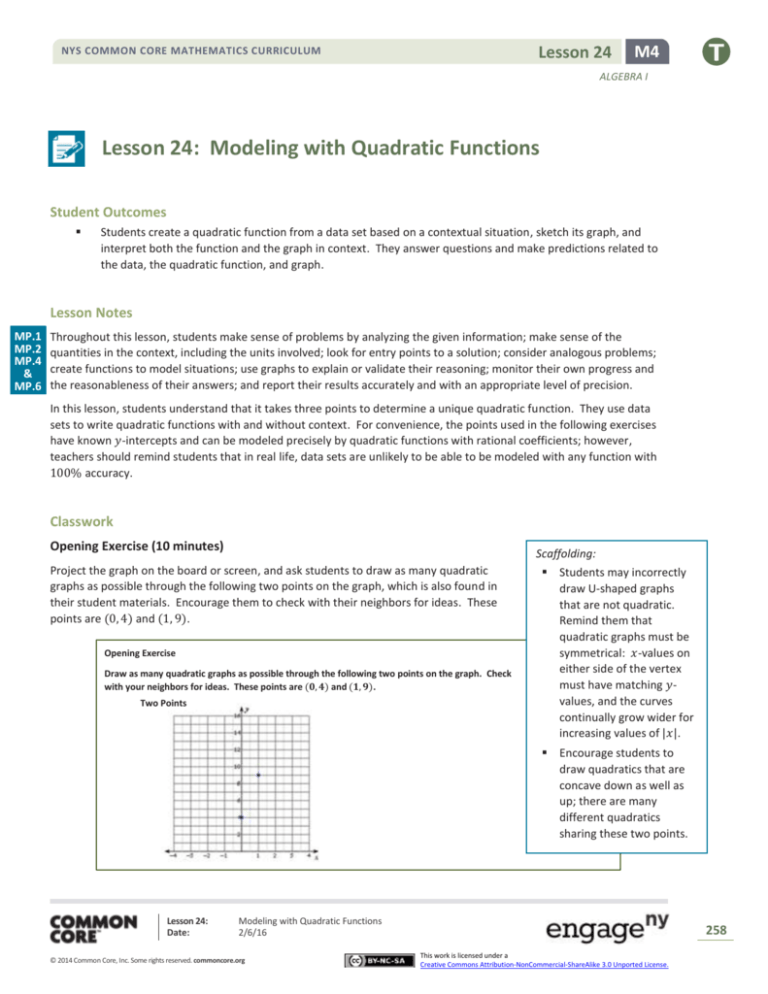
Project the graph on the board or screen, and ask students to draw as many quadratic
graphs as possible through the following two points on the graph, which is also found in
their student materials. Encourage them to check with their neighbors for ideas. These
points are (0, 4) and (1, 9).
Opening Exercise
Draw as many quadratic graphs as possible through the following two points on the graph. Check
with your neighbors for ideas. These points are (𝟎, 𝟒) and (𝟏, 𝟗).
Two Points
 Students may incorrectly
draw U-shaped graphs
that are not quadratic.
Remind them that
quadratic graphs must be
symmetrical: 𝑥-values on
either side of the vertex
must have matching 𝑦values, and the curves
continually grow wider for
increasing values of |𝑥|.
 Encourage students to
draw quadratics that are
concave down as well as
up; there are many
different quadratics
sharing these two points.
Lesson 24:
Date:
Modeling with Quadratic Functions
2/6/16
© 2014 Common Core, Inc. Some rights reserved. commoncore.org
258
This work is licensed under a
Creative Commons Attribution-NonCommercial-ShareAlike 3.0 Unported License.
Lesson 24
NYS COMMON CORE MATHEMATICS CURRICULUM
M4
ALGEBRA I
After a few minutes, gather the class together, and have students share some of their graphs. You might have three or
four students come to the board and sketch one of their graphs, each in a different color. There are an infinite number
of solutions. Make sure that some of the sketches have one of the points as a vertex and that some open up and some
down.
Now, introduce a third point and ask students to repeat the exercise. Now the points are (0, 4), (1, 9), and (−3, 1).
Three Points
Scaffolding:
Unlike in the previous example,
advanced students may notice
that when three points are
known, the value of the
“second difference” is fixed;
therefore, the quadratic
function is uniquely defined.

Ultimately, students should conclude that only
one quadratic graph can pass through all three
points simultaneously. Therefore, it requires no
less than three points to determine a quadratic
function.
Students may be curious about what happens if a
fourth point is introduced. Add a fourth point in
two different places, and have them study the
possibilities. Try adding a point in another color
that is on the quadratic graph, (−1, 1), and then
add one that is not, (2, 5).
Scaffolding:
 Students may remember from earlier lessons that in quadratic
equations, “second differences” are equal. This supports the idea that
any number of quadratic equations can be drawn through two points
because the value of the second difference is not well defined. Here is
an example showing a quadratic function with its 1st and 2nd
differences.
𝒙𝟐 − 𝒙𝟏
1
1
1
1
Fourth Point #1
𝒇(𝒙) = −𝟓(𝒙 − 𝟏)𝟐 + 𝟗
1st 𝒇 Diff
𝒙
𝒚
𝒚𝟐 − 𝒚 𝟏
0
4
1
9
5
2
4
−5
3
−11
−15
4
−36
−25
2nd Diff
−10
−10
−10
Point out that the differences in the 𝑥-values do not have to be 1 but must
be regular. Ask why.
 Why must the differences in the 𝑥-values for the selected data points
be at regular intervals?


 If the first differences represent the average rate of change for an
interval (slope), how would you describe the second differences?


Lesson 24:
Date:
We are comparing rates of change. We need a constant change in
𝑥 so that we are comparing equal intervals.
They can be described as the average rate of change of the slope,
or the slope of the slope.
Modeling with Quadratic Functions
2/6/16
© 2014 Common Core, Inc. Some rights reserved. commoncore.org
259
This work is licensed under a
Creative Commons Attribution-NonCommercial-ShareAlike 3.0 Unported License.
Lesson 24
NYS COMMON CORE MATHEMATICS CURRICULUM
M4
ALGEBRA I
Fourth Point #2


Explain that a fourth point, in this case (2, 5), may either belong to the quadratic (see: Fourth Point #1 graph) or not
(see: Fourth Point #2 graph), but the function has already been determined by the first three (blue) points.
Example (10 minutes)
Example
Use the example with the blue points (𝟎, 𝟒), (𝟏, 𝟗), and (−𝟑, 𝟏) from above to write the equation for the quadratic
containing the three points.
Demonstrate for students how, if we know the 𝑦-intercept and two other points for a quadratic, we can form a system
of linear equations to determine the standard form of the quadratic function defined by those points. Use the example
with the blue points above: (0, 4), (1, 9), and (−3, 1).

Notice that we have the 𝑦-intercept, which allows us to find the value of 𝑐 quickly and first. After that, we can
substitute the other two coordinates into the equation, giving us two linear equations to solve simultaneously.
Using (0, 4)
Using (1, 9)
𝑓(𝑥) = 𝑎𝑥 2 + 𝑏𝑥 + 𝑐
Using (−3, 1)
𝑓(𝑥) = 𝑎𝑥 2 + 𝑏𝑥 + 4
4 = 𝑎(0)2 + 𝑏(0) + 𝑐
9 = 𝑎(1)2 + 𝑏(1) + 4
4=𝑐
9=𝑎+𝑏+4
𝑎+𝑏 =5

𝑓(𝑥) = 𝑎𝑥 2 + 𝑏𝑥 + 4
Since 𝑐 = 4, the resulting system has two variables: {
𝑓(𝑥) = 𝑎(−3)2 + 𝑏(−3) + 4
1 = 9𝑎 − 3𝑏 + 4
9𝑎 − 3𝑏 = −3
𝑎+𝑏 =5
. Use substitution or elimination to
9𝑎 − 3𝑏 = −3
determine that 𝑎 = 1 and 𝑏 = 4.

Substitute 𝑎 = 1, 𝑏 = 4, and 𝑐 = 4 into standard form: 𝑓(𝑥) = 𝑥 2 + 4𝑥 + 4 is the quadratic function that
contains the given points.
Demonstrate that the graph of the function we just found does, in fact, pass through all three points by showing the
graph on the board or screen.
Lesson 24:
Date:
Modeling with Quadratic Functions
2/6/16
© 2014 Common Core, Inc. Some rights reserved. commoncore.org
260
This work is licensed under a
Creative Commons Attribution-NonCommercial-ShareAlike 3.0 Unported License.
Lesson 24
NYS COMMON CORE MATHEMATICS CURRICULUM
M4
ALGEBRA I

Notice that in the graph below, we have included the two different fourth points from the Opening Exercise,
(−1, 1) and (2, 5). Clearly (−1, 1) is on the graph of the function, but (2, 5) is not.
Exercise 1 (10 minutes)
Have students complete the following exercise independently.
Exercise 1
Write in standard form the quadratic function defined by the points (𝟎, 𝟓), (𝟓, 𝟎), and (𝟑, −𝟒).
Using (𝟎, 𝟓)
Using (𝟓, 𝟎)
𝒇(𝒙) = 𝒂𝒙𝟐 + 𝒃𝒙 + 𝒄
Using (𝟑, −𝟒)
𝒇(𝒙) = 𝒂𝒙𝟐 + 𝒃𝒙 + 𝟓
𝟐
𝟐
𝟓 = 𝒂(𝟎) + 𝒃(𝟎) + 𝒄
𝒇(𝒙) = 𝒂𝒙𝟐 + 𝒃𝒙 + 𝟓
𝟎 = 𝒂(𝟓) + 𝒃(𝟓) + 𝟓
𝟓=𝒄
𝟎 = 𝟐𝟓𝒂 + 𝟓𝒃 + 𝟓
−𝟒 = 𝒂(𝟑)𝟐 + 𝒃(𝟑) + 𝟓
−𝟒 = 𝟗𝒂 + 𝟑𝒃 + 𝟓
𝟐𝟓𝒂 + 𝟓𝒃 = −𝟓
𝟗𝒂 + 𝟑𝒃 = −𝟗
𝟓𝒂 + 𝒃 = −𝟏
𝟑𝒂 + 𝒃 = −𝟑
𝟓𝒂 + 𝒃 = −𝟏
Since 𝒄 = 𝟓, the resulting system has two variables: {
.
𝟑𝒂 + 𝒃 = −𝟑
Use substitution or elimination, and find that 𝒂 = 𝟏 and 𝒃 = −𝟔.
Substitute 𝒂 = 𝟏, 𝒃 = −𝟔, and 𝒄 = 𝟓 into standard form: 𝒇(𝒙) = 𝒙𝟐 − 𝟔𝒙 + 𝟓 is the quadratic function that contains the
given points.
Exercise 2 (10 minutes)
Have students work with a partner or in small groups to write the quadratic equation for the function defined by the
following data set. Have them read the description of the experiment and study the collected data. Then, use the
guiding questions to walk the students through the process of writing the quadratic equation to represent the data.
Lesson 24:
Date:
Modeling with Quadratic Functions
2/6/16
© 2014 Common Core, Inc. Some rights reserved. commoncore.org
261
This work is licensed under a
Creative Commons Attribution-NonCommercial-ShareAlike 3.0 Unported License.
Lesson 24
NYS COMMON CORE MATHEMATICS CURRICULUM
M4
ALGEBRA I
Exercise 2
Louis dropped a watermelon from the roof of a tall building. As it was falling, Amanda and Martin were on the ground
with a stopwatch. As Amanda called the seconds, Martin recorded the floor the watermelon was passing. They then
measured the number of feet per floor and put the collected data into this table. Write a quadratic function to model the
following table of data relating the height of the watermelon (distance in feet from the ground) to the number of seconds
that had passed.
Height (distance from the ground) for a watermelon that was dropped from a tall building
Time (𝒕)
𝟎
𝟏
𝟐
𝟑
𝟒
Height 𝒇(𝒕)
𝟑𝟎𝟎
𝟐𝟖𝟒
𝟐𝟑𝟔
𝟏𝟓𝟔
𝟒𝟒
a.
How do we know this data will be represented by a quadratic function?
The relationship between height and time for all free-falling objects is represented by a quadratic equation.
Also, we can see mathematically that the function values have a first difference of −𝟏𝟔, −𝟒𝟖, −𝟖𝟎, and
−𝟏𝟏𝟐. The second differences are constant at −𝟑𝟐.
b.
Do we need to use all five data points to write the equation?
No, only three are needed.
c.
Are there any points that are particularly useful? Does it matter which we use?
(𝟎, 𝟑𝟎𝟎) is useful because it is the 𝒚-intercept. We will need to use (𝟎, 𝟑𝟎𝟎), but the other two can be
selected based on efficiency (the least messy or smallest numbers).
Encourage different groups of students to use different sets of three points and then compare their results.
Use (𝟎, 𝟑𝟎𝟎)
Use (𝟏, 𝟐𝟖𝟒)
𝟐
𝒇(𝒕) = 𝒂𝒕 + 𝒃𝒕 + 𝒄
𝟐
Use (𝟐, 𝟐𝟑𝟔)
𝟐
𝒇(𝒕) = 𝒂𝒕𝟐 + 𝒃𝒕 + 𝒄
𝒇(𝒕) = 𝒂𝒕 + 𝒃𝒕 + 𝒄
𝟐
𝟑𝟎𝟎 = 𝒂(𝟎) + 𝒃(𝟎) + 𝒄
𝟐𝟖𝟒 = 𝒂(𝟏) + 𝒃(𝟏) + 𝟑𝟎𝟎
𝟐𝟑𝟔 = 𝒂(𝟐)𝟐 + 𝒃(𝟐) + 𝟑𝟎𝟎
𝟑𝟎𝟎 = 𝒄
−𝟏𝟔 = 𝒂 + 𝒃
−𝟔𝟒 = 𝟒𝒂 + 𝟐𝒃
−𝟏𝟔 = 𝒂 + 𝒃
Since 𝒄 = 𝟑𝟎𝟎, the resulting system has two variables: {
.
−𝟔𝟒 = 𝟒𝒂 + 𝟐𝒃
Use substitution or elimination and find that 𝒂 = −𝟏𝟔 and 𝒃 = 𝟎.
Substitute 𝒂 = −𝟏𝟔, 𝒃 = 𝟎, and 𝒄 = 𝟑𝟎𝟎 into standard form: 𝒇(𝒕) = −𝟏𝟔𝒕𝟐 + 𝟑𝟎𝟎.
Note: The same values for 𝑎, 𝑏, and 𝑐 will occur no matter which points are used to write the function. However, the
point (0, 300) is particularly useful because it solves the system for 𝑐 right away. Not using (0, 300) first means that the
students will need to solve a 3 × 3 system of equations. Students learn in Grade 8 to solve a 2 × 2 system of equations
(8.EE.C.8), but solving a 3 × 3 system is considered an advanced topic in Algebra II (A.APR.D.7). Students could also
point out that smaller values for 𝑡 yield smaller coefficients for the system, making it easier to solve.
d.
How does this equation for the function match up with what you learned about physics in Lesson 23? Is there
a more efficient way to find this equation?
It matches perfectly. This equation shows that the initial position (height) of the object is 𝟑𝟎𝟎 𝐟𝐭. and that the
initial velocity is 𝟎. It correctly uses −𝟏𝟔 as the leading coefficient. We could have written the equation
directly from the information provided since we already know the initial height and velocity.
Lesson 24:
Date:
Modeling with Quadratic Functions
2/6/16
© 2014 Common Core, Inc. Some rights reserved. commoncore.org
262
This work is licensed under a
Creative Commons Attribution-NonCommercial-ShareAlike 3.0 Unported License.
NYS COMMON CORE MATHEMATICS CURRICULUM
Lesson 24
M4
ALGEBRA I
e.
Can you use your quadratic function to predict at what time, t, the watermelon will hit the ground (i.e.,
𝒇(𝒕) = 𝟎)?
Yes.
𝒇(𝒕) = −𝟏𝟔𝒕𝟐 + 𝟑𝟎𝟎
𝟎 = −𝟏𝟔𝒕𝟐 + 𝟑𝟎𝟎
−𝟑𝟎𝟎 = −𝟏𝟔𝒕𝟐
𝟏𝟖. 𝟕𝟓 = 𝒕𝟐
±𝟒. 𝟑𝟑 ≈ 𝒕
So, the watermelon hit the ground after about 𝟒. 𝟑𝟑 𝐬𝐞𝐜.
Closing (1 minute)
To determine a unique quadratic function from a table or graph, we must know at least three distinct points.
Lesson Summary
We can create a quadratic function from a data set based on a contextual situation, sketch its graph, and interpret
both the function and the graph in context. We can then answer questions and make predictions related to the
data, the quadratic function, and graph.
To determine a unique quadratic function from a table or graph, we must know at least three distinct points.
Exit Ticket (4 minutes)
Lesson 24:
Date:
Modeling with Quadratic Functions
2/6/16
© 2014 Common Core, Inc. Some rights reserved. commoncore.org
263
This work is licensed under a
Creative Commons Attribution-NonCommercial-ShareAlike 3.0 Unported License.
Lesson 24
NYS COMMON CORE MATHEMATICS CURRICULUM
M4
ALGEBRA I
Name ___________________________________________________
Date____________________
Lesson 24: Modeling with Quadratic Functions
Exit Ticket
Write a quadratic function from the following table of data.
Fertilizer Impact on Corn Yields
0
100 200
Fertilizer, 𝑥 (kg/m2 )
4.7
8.7 10.7
Corn Yield, 𝑦 (1000 bushels)
Lesson 24:
Date:
300
10.7
400
8.7
Modeling with Quadratic Functions
2/6/16
© 2014 Common Core, Inc. Some rights reserved. commoncore.org
264
This work is licensed under a
Creative Commons Attribution-NonCommercial-ShareAlike 3.0 Unported License.
Lesson 24
NYS COMMON CORE MATHEMATICS CURRICULUM
M4
ALGEBRA I
Exit Ticket Sample Solutions
Write a quadratic function from the following table of data.
Fertilizer Impact on Corn Yields
𝟎
𝟏𝟎𝟎
Fertilizer, 𝒙 (𝐤𝐠/𝐦𝟐)
Corn Yield, 𝒚 (1000 bushels)
𝟒. 𝟕
𝟖. 𝟕
𝟐𝟎𝟎
𝟏𝟎. 𝟕
𝟑𝟎𝟎
𝟏𝟎. 𝟕
𝟒𝟎𝟎
𝟖. 𝟕
Using the three points:
Use (𝟎, 𝟒. 𝟕)
Use (𝟏𝟎𝟎, 𝟖. 𝟕)
𝒇(𝒙) = 𝒂𝒙𝟐 + 𝒃𝒙 + 𝒄
𝒇(𝒙) = 𝒂𝒙𝟐 + 𝒃𝒙 + 𝒄
𝟒. 𝟕 = 𝒂(𝟎)𝟐 + 𝒃(𝟎) + 𝒄
Use (𝟐𝟎𝟎, 𝟏𝟎. 𝟕)
𝒇(𝒙) = 𝒂𝒙𝟐 + 𝒃𝒙 + 𝒄
𝟖. 𝟕 = 𝒂(𝟏𝟎𝟎)𝟐 + 𝒃(𝟏𝟎𝟎) + 𝟒. 𝟕
𝟒 = 𝟏𝟎, 𝟎𝟎𝟎𝒂 + 𝟏𝟎𝟎𝒃
𝟒. 𝟕 = 𝒄
Since 𝒄 = 𝟒. 𝟕, the resulting system has two variables: {
Use substitution or elimination and find that 𝒂 =
𝟏𝟎. 𝟕 = 𝒂(𝟐𝟎𝟎)𝟐 + 𝒃(𝟐𝟎𝟎) + 𝟒. 𝟕
𝟔 = 𝟒𝟎, 𝟎𝟎𝟎𝒂 + 𝟐𝟎𝟎𝒃
𝟒 = 𝟏𝟎, 𝟎𝟎𝟎𝒂 + 𝟏𝟎𝟎𝒃
.
𝟔 = 𝟒𝟎, 𝟎𝟎𝟎𝒂 + 𝟐𝟎𝟎𝒃
−𝟏
𝟏
= −𝟎. 𝟎𝟎𝟎𝟏 and 𝒃 =
= 𝟎. 𝟎𝟓.
𝟏𝟎,𝟎𝟎𝟎
𝟐𝟎
Substitute 𝒂 = −𝟎. 𝟎𝟎𝟎𝟏, 𝒃 = 𝟎. 𝟎𝟓, and 𝒄 = 𝟒. 𝟕 into standard form: 𝒇(𝒙) = −𝟎. 𝟎𝟎𝟎𝟏𝒙𝟐 + 𝟎. 𝟎𝟓𝒙 + 𝟒. 𝟕.
Problem Set Sample Solutions
1.
Write a quadratic function to fit the following points, and state the 𝒙-values for both roots. Then, sketch the graph
to show that the equation includes the three points.
Using the three points:
Use (𝟎, 𝟒)
Use (−𝟐, 𝟎)
𝒇(𝒙) = 𝒂𝒙𝟐 + 𝒃𝒙 + 𝒄
Use (𝟏, 𝟑)
𝒇(𝒙) = 𝒂𝒙𝟐 + 𝒃𝒙 + 𝒄
𝟐
𝟒 = 𝒂(𝟎) + 𝒃(𝟎) + 𝒄
𝟒=𝒄
𝒇(𝒙) = 𝒂𝒙𝟐 + 𝒃𝒙 + 𝒄
𝟐
𝟎 = 𝒂(−𝟐) + 𝒃(−𝟐) + 𝟒
−𝟒 = 𝟒𝒂 − 𝟐𝒃
𝟑 = 𝒂(𝟏)𝟐 + 𝒃(𝟏) + 𝟒
−𝟏 = 𝒂 + 𝒃
−𝟒 = 𝟒𝒂 − 𝟐𝒃
Since 𝒄 = 𝟒, the resulting system has two variables: {
.
−𝟏 = 𝒂 + 𝒃
Use substitution or elimination and find that 𝒂 = −𝟏 and 𝒃 = 𝟎.
Substitute 𝒂 = −𝟏, 𝒃 = 𝟎, and 𝒄 = 𝟒 into standard form: 𝒇(𝒙) = −𝒙𝟐 + 𝟒.
Lesson 24:
Date:
Modeling with Quadratic Functions
2/6/16
© 2014 Common Core, Inc. Some rights reserved. commoncore.org
265
This work is licensed under a
Creative Commons Attribution-NonCommercial-ShareAlike 3.0 Unported License.
Lesson 24
NYS COMMON CORE MATHEMATICS CURRICULUM
M4
ALGEBRA I
2.
Write a quadratic function to fit the following points: (𝟎, 𝟎. 𝟏𝟕𝟓), (𝟐𝟎, 𝟑. 𝟓𝟕𝟓), (𝟑𝟎, 𝟒. 𝟔𝟕𝟓).
Use (𝟎, 𝟎. 𝟏𝟕𝟓)
Use (𝟐𝟎, 𝟑. 𝟓𝟕𝟓)
𝒇(𝒙) = 𝒂𝒙𝟐 + 𝒃𝒙 + 𝒄
Use (𝟑𝟎, 𝟒. 𝟔𝟕𝟓)
𝒇(𝒙) = 𝒂𝒙𝟐 + 𝒃𝒙 + 𝒄
𝟐
𝟒. 𝟔𝟕𝟓 = 𝒂(𝟑𝟎)𝟐 + 𝒃(𝟑𝟎) + 𝟎. 𝟏𝟕𝟓
𝟐
𝒇(𝒙) = 𝒂𝒙 + 𝒃𝒙 + 𝒄
𝟑. 𝟓𝟕𝟓 = 𝒂(𝟐𝟎) + 𝒃(𝟐𝟎) + 𝟎. 𝟏𝟕𝟓
𝟎. 𝟏𝟕𝟓 = 𝒂(𝟎)𝟐 + 𝒃(𝟎) + 𝒄
𝟒. 𝟓 = 𝟗𝟎𝟎𝒂 + 𝟑𝟎𝒃
𝟑. 𝟒 = 𝟒𝟎𝟎𝒂 + 𝟐𝟎𝒃
𝟎. 𝟏𝟕𝟓 = 𝒄
𝟑. 𝟒 = 𝟒𝟎𝟎𝒂 + 𝟐𝟎𝒃
Since 𝒄 = 𝟎. 𝟏𝟕𝟓, the resulting system has two variables: {
.
𝟒. 𝟓 = 𝟗𝟎𝟎𝒂 + 𝟑𝟎𝒃
Use substitution or elimination and find that 𝒂 = −𝟎. 𝟎𝟎𝟐 and 𝒃 = 𝟎. 𝟐𝟏.
Substitute 𝒂 = −𝟎. 𝟎𝟎𝟐, 𝒃 = 𝟎. 𝟐𝟏, and 𝒄 = 𝟎. 𝟏𝟕𝟓 into standard form:
𝒇(𝒙) = −𝟎. 𝟎𝟎𝟐𝒙𝟐 + 𝟎. 𝟐𝟏𝒙 + 𝟎. 𝟏𝟕𝟓.
Lesson 24:
Date:
Modeling with Quadratic Functions
2/6/16
© 2014 Common Core, Inc. Some rights reserved. commoncore.org
266
This work is licensed under a
Creative Commons Attribution-NonCommercial-ShareAlike 3.0 Unported License.
Lesson 24
NYS COMMON CORE MATHEMATICS CURRICULUM
M4
ALGEBRA I
Lagrange’s Interpolation Method: An Extension for Accelerated Students
Lagrange’s Interpolation Method allows mathematicians to write a polynomial from a given set of points. Because three
points determine a unique quadratic function, students can use interpolation to write a quadratic function without
having to solve a system of equations to find the coefficients.
Given the points (𝑎, 𝑏), (𝑐, 𝑑), (𝑒, 𝑓), the quadratic function defined by these points can be written as follows:
𝑓(𝑥) = 𝑏 ∙
(𝑥 − 𝑐)(𝑥 − 𝑒)
(𝑥 − 𝑎)(𝑥 − 𝑒)
(𝑥 − 𝑎)(𝑥 − 𝑐)
+𝑑∙
+𝑓∙
.
(𝑎 − 𝑐)(𝑎 − 𝑒)
(𝑐 − 𝑎)(𝑐 − 𝑒)
(𝑒 − 𝑎)(𝑒 − 𝑐)
This works because, for each 𝑥 substituted into the function, two of the terms disappear by the zero–multiplication rule,
and the third term divides to𝑓(𝑥) ∙ 1. For example, write the quadratic function uniquely defined by the points: (−1, 2),
(2, 23), (−4, −1).
𝑓(𝑥) = 2 ∙
Then, 𝑓(2) = 2 ∙
(2−2)(2+4)
(−3)(3)
and 𝑓(2) = 0 + 23 ∙
(3)(6)
(3)(6)
(𝑥 − 2)(𝑥 + 4)
(𝑥 + 1)(𝑥 + 4)
(𝑥 + 1)(𝑥 − 2)
+ 23 ∙
−1∙
;
(−3)(3)
(3)(6)
(−3)(−6)
+ 23 ∙
(2+1)(2+4)
(3)(6)
−1∙
(2+1)(2−2)
(−3)(−6)
,
− 0,
so 𝑓(2) = 23 ∙ 1 = 23.
This process can be repeated for each of the three points, and so this function is clearly a degree two polynomial
containing the three given points. This form may be considered perfectly acceptable; however, by multiplying out and
collecting like terms, we can rewrite this function in standard form.
𝑓(𝑥) =
−2 2
23 2
1 2
(𝑥 + 2𝑥 − 8) +
(𝑥 + 5𝑥 + 4) −
(𝑥 − 𝑥 − 2)
9
18
18
18𝑓(𝑥) = −4𝑥 2 − 8𝑥 + 32 + 23𝑥 2 + 115𝑥 + 92 − 𝑥 2 + 𝑥 + 2
18𝑓(𝑥) = 18𝑥 2 + 108𝑥 + 126
𝑓(𝑥) = 𝑥 2 + 6𝑥 + 7
For students who love a challenge, design a short set of exercises with which accelerated students may practice
interpolation. These exercises should not necessarily reduce to integer or even rational coefficients in standard form,
and students may want to consider the potential pros and cons of leaving the function in its original interpolated form.
Lesson 24:
Date:
Modeling with Quadratic Functions
2/6/16
© 2014 Common Core, Inc. Some rights reserved. commoncore.org
267
This work is licensed under a
Creative Commons Attribution-NonCommercial-ShareAlike 3.0 Unported License.