G563
Department of Geological Sciences | P. David Polly
1.
Familiarize yourself with the following functions: a.
DiversityPlot[] b.
DiversityTable[] c.
CohortAnalysis[] d.
LetThereBeLight[]
2.
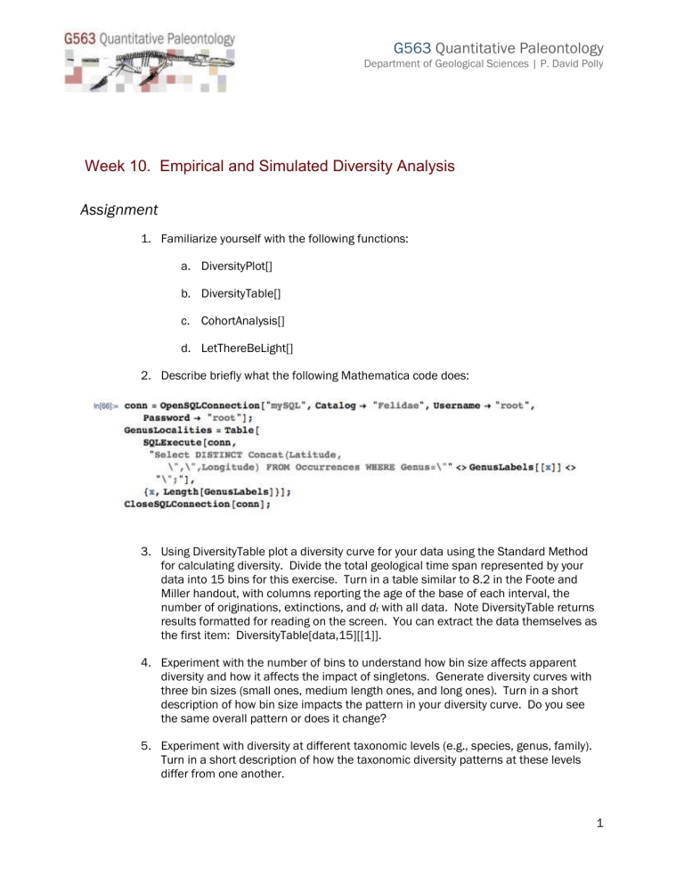
Describe briefly what the following Mathematica code does:
3.
Using DiversityTable plot a diversity curve for your data using the Standard Method for calculating diversity. Divide the total geological time span represented by your data into 15 bins for this exercise. Turn in a table similar to 8.2 in the Foote and
Miller handout, with columns reporting the age of the base of each interval, the number of originations, extinctions, and d t
with all data. Note DiversityTable returns results formatted for reading on the screen. You can extract the data themselves as the first item: DiversityTable[data,15][[1]].
4.
Experiment with the number of bins to understand how bin size affects apparent diversity and how it affects the impact of singletons. Generate diversity curves with three bin sizes (small ones, medium length ones, and long ones). Turn in a short description of how bin size impacts the pattern in your diversity curve. Do you see the same overall pattern or does it change?
5.
Experiment with diversity at different taxonomic levels (e.g., species, genus, family).
Turn in a short description of how the taxonomic diversity patterns at these levels differ from one another.
1

6.
Turn in a short description (and figure) of the history of taxonomic diversity in your group. For example, has the group increased in diversity or declined? Were there particular points in geological time when their diversity substantially increased or decreased? Are those times associated with other events with which you are aware?
(e.g., asteroid impacts, climate changes, origin of plant groups, etc.). What are the rates of origination and extinction in your group?
7.
Perform a cohort analysis at two different census points, one when there was low diversity and one when there was higher diversity. (if your group increases in diversity toward the present, pick an earlier time even though diversity might not have been as high then). What do the survivorship curves tell you?
8.
Use the LetThereBeLight[] function to simulate the evolution of clades and to see how different parameters affect patterns of diversity. a.
Evaluate the chances of long-term success of a clade when origination and extinction are equal to 0.5. To do this, run ten simulations with time set to
100 million years, number of lineages at the start of the simulation set to 1, and λ and μ both set to 0.5. Record the time of extinction of the last surviving lineage in each simulation. Report the median duration of your clade and the proportion of times it becomes extinct before the simulation ends (i.e, before
100 million years have elapsed). The proportion is an estimate of the probability that the clade becomes extinct at or before time zero. Using the equations in Raup’s appendix, what are the expected median duration and probability of extinction before time zero? b.
Evaluate the variation in the estimated origination (λ) and extinction (μ) parameters by running ten simulations with time set to 100 million years, number of lineages at the start of the simulation set to 1, and λ and μ both set to 0.5. Record the estimated values of λ and μ for each simulation. What are the ranges of the two parameters across the simulations? Their means?
The standard errors on these parameters can be estimated from the standard deviations of the simulated data. What are the standard errors? c.
Repeat the evaluation of λ and μ, but this time run ten simulations for 100 million years with 10 starting lineages and λ and μ both equal to 0.75. What happens to the standard error of λ and μ? Why? d.
Evaluate the effect of λ and μ on median duration of each species lineage.
Run 10 simulations for 100 million years with 10 starting lineages for λ and μ
= 0.25, λ and μ = 0.5, and λ and μ = 0.75. For each set of ten simulations, record the median lineage duration, and find the average median duration for each set. Graph the relationship between the value of λ and μ and the average median duration. What is the relationship and why? e.
Evaluate the effect of (λ – μ) on diversification. Using a similar procedure as in part d, run ten simulations for 100 million years with three starting lineages. For each set of ten simulations, set μ = 0.5 and then change λ from
0.45 to 0.50, to 0.55. Record the total number of lineages, and find the average for each block of ten simulations. (note: you may encounter an error when all lineages become extinct in the first generation of the simulation).
2