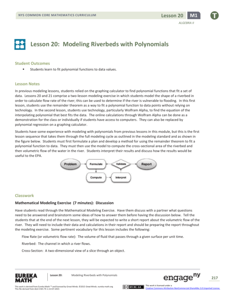
NYS COMMON CORE MATHEMATICS CURRICULUM
Lesson 20
M1
ALGEBRA II
Lesson 20: Modeling Riverbeds with Polynomials
Student Outcomes

Students learn to fit polynomial functions to data values.
Lesson Notes
In previous modeling lessons, students relied on the graphing calculator to find polynomial functions that fit a set of
data. Lessons 20 and 21 comprise a two-lesson modeling exercise in which students model the shape of a riverbed in
order to calculate flow rate of the river; this can be used to determine if the river is vulnerable to flooding. In this first
lesson, students use the remainder theorem as a way to fit a polynomial function to data points without relying on
technology. In the second lesson, students use technology, particularly Wolfram Alpha, to find the equation of the
interpolating polynomial that best fits the data. The online calculations through Wolfram Alpha can be done as a
demonstration for the class or individually if students have access to computers. They can also be replaced by
polynomial regression on a graphing calculator.
Students have some experience with modeling with polynomials from previous lessons in this module, but this is the first
lesson sequence that takes them through the full modeling cycle as outlined in the modeling standard and as shown in
the figure below. Students must first formulate a plan and develop a method for using the remainder theorem to fit a
polynomial function to data. They must then use the model to compute the cross-sectional area of the riverbed and
then volumetric flow of the water in the river. Students interpret their results and discuss how the results would be
useful to the EPA.
Classwork
Mathematical Modeling Exercise (7 minutes): Discussion
Have students read through the Mathematical Modeling Exercise. Have them discuss with a partner what questions
need to be answered and brainstorm some ideas of how to answer them before having the discussion below. Tell the
students that at the end of the next lesson, they will be expected to write a short report about the volumetric flow of the
river. They will need to include their data and calculations in their report and should be preparing the report throughout
the modeling exercise. Some pertinent vocabulary for this lesson includes the following:
Flow Rate (or volumetric flow rate): The volume of fluid that passes through a given surface per unit time.
Riverbed: The channel in which a river flows.
Cross-Section: A two-dimensional view of a slice through an object.
Lesson 20:
Modeling Riverbeds with Polynomials
This work is derived from Eureka Math ™ and licensed by Great Minds. ©2015 Great Minds. eureka-math.org
This file derived from ALG II-M1-TE-1.3.0-07.2015
217
This work is licensed under a
Creative Commons Attribution-NonCommercial-ShareAlike 3.0 Unported License.
Lesson 20
NYS COMMON CORE MATHEMATICS CURRICULUM
M1
ALGEBRA II
In order for students to formulate a plan for modeling the shape of the
riverbed, they must change their perspective from working with a threedimensional idea of a river to the idea of working solely with a two-dimensional
cross section. A figure such as the one to the right helps students see how the
cross-sectional slice of the river relates to the river as a whole. The lower edge
of the cross-section (shown in darker blue) is the curve that we need to find
that goes through the given data points.

Read through the statement of the Mathematical Modeling Exercise.
What is our goal?


How can we estimate the flow rate of water?


We need to find the flow rate of water through the riverbed.
We need the area of the cross-section and the current speed of the water. Then the flow rate is the
product of the cross-sectional area (in square feet) and the speed of the water (in feet per second).
To estimate the area of the cross-section, what information do we need?

We need enough data points to make a good estimate.

To gather enough data points, we will need to make an assumption that the riverbed changes smoothly
between the data points we have. With that assumption, we could estimate other data points by
approximating the curve of the cross-section using a polynomial function.

What is our first task?


We need to find a polynomial function to fit the data.
Draw the graph of a polynomial function that passes through the 5 given data points.
Mathematical Modeling Exercise
The Environmental Protection Agency (EPA) is studying the flow of a river in order to establish flood zones. The EPA hired
a surveying company to determine the flow rate of the river, measured as volume of water per minute. The firm set up a
coordinate system and found the depths of the river at five locations as shown on the graph below. After studying the
data, the firm decided to model the riverbed with a polynomial function and divide the cross-sectional area into six
regions that are either trapezoidal or triangular so that the overall area can be easily estimated. The firm needs to
approximate the depth of the river at two more data points in order to do this.
Lesson 20:
Modeling Riverbeds with Polynomials
This work is derived from Eureka Math ™ and licensed by Great Minds. ©2015 Great Minds. eureka-math.org
This file derived from ALG II-M1-TE-1.3.0-07.2015
218
This work is licensed under a
Creative Commons Attribution-NonCommercial-ShareAlike 3.0 Unported License.
Lesson 20
NYS COMMON CORE MATHEMATICS CURRICULUM
M1
ALGEBRA II
Draw the four trapezoids and two triangles that will be used to estimate the cross-sectional area of the riverbed.

We have five data points. What information are we missing?


How can we find the missing values?

MP.1

Find a polynomial function 𝑃 that fits the given data and then use its equation to find 𝑃(40) and
𝑃(80), which should approximate the depths at 𝑥 = 40 and 𝑥 = 80.
What is the lowest-degree polynomial that could be used to model this data?


The depths at 𝑥 = 40 and 𝑥 = 80
Degree four, because we have three relative maximum and minimum points.
What constraints must our polynomial meet?

𝑃(0) = 0, 𝑃(20) = −20, 𝑃(60) = −15, 𝑃(100) = −25, and 𝑃(120) = 0
Example 1 (12 minutes)
Work this example out two ways. First, let students find the equation by setting up a system of equations (as in
Lesson 1). Then, demonstrate how the remainder theorem can be used to find the polynomial.

Before trying to find a polynomial function whose graph goes through all five points, let’s try a simpler problem
and find a polynomial whose graph goes through just three of the points: (0,28), (2,0), and (8, 12).
Display these three points on a coordinate grid to use as reference through this discussion.

Will the polynomial function that we find through these points be linear?


What do you think is the lowest-degree polynomial we can find that passes through the three points (0,28),
(2,0), and (8, 12)? (Remind students to look at the locations of these points in the plane as they decide on the
lowest possible degree.)


No, looking at the graph, we see that the points do not lie on a line.
It appears that we could fit a quadratic polynomial to these points; that is, they seem to lie on a
parabola.
Try to find a quadratic polynomial whose graph passes through these points. (Give students a hint to find a
system of equations by plugging in 𝑥 and 𝑃(𝑥) values into the equation 𝑃(𝑥) = 𝑎𝑥 2 + 𝑏𝑥 + 𝑐 as they did in
Lesson 1.)
Lesson 20:
Modeling Riverbeds with Polynomials
This work is derived from Eureka Math ™ and licensed by Great Minds. ©2015 Great Minds. eureka-math.org
This file derived from ALG II-M1-TE-1.3.0-07.2015
219
This work is licensed under a
Creative Commons Attribution-NonCommercial-ShareAlike 3.0 Unported License.
Lesson 20
NYS COMMON CORE MATHEMATICS CURRICULUM
M1
ALGEBRA II
Allow students time to work, and then discuss the process as a class.
Example 1
Find a polynomial 𝑷 such that 𝑷(𝟎) = 𝟐𝟖, 𝑷(𝟐) = 𝟎, and 𝑷(𝟖) = 𝟏𝟐.
Since 𝑷(𝟎) = 𝟐𝟖, 𝒄 = 𝟐𝟖 →
𝑷(𝒙) = 𝒂𝒙𝟐 + 𝒃𝒙 + 𝟐𝟖
Since 𝑷(𝟐) = 𝟎
→
𝟒𝒂 + 𝟐𝒃 + 𝟐𝟖 = 𝟎, so 𝟐𝒂 + 𝒃 = −𝟏𝟒
(1)
Since 𝑷(𝟖) = 𝟏𝟐
→
𝟔𝟒𝒂 + 𝟖𝒃 + 𝟐𝟖 = 𝟏𝟐, so 𝟖𝒂 + 𝒃 = −𝟐
(2)
Subtract (1) from (2).
→
𝟔𝒂 = 𝟏𝟐, so 𝒂 = 𝟐
Substitute to find 𝒃.
→
𝟐(𝟐) + 𝒃 = −𝟏𝟒, so 𝒃 = −𝟏𝟖
𝑷(𝒙) = 𝟐𝒙𝟐 − 𝟏𝟖𝒙 + 𝟐𝟖
Have students check their equation by finding 𝑃(0), 𝑃(2), and 𝑃(8) and showing that 𝑃(0) = 28, 𝑃(2) = 0, and
𝑃(8) = 12. Now work the problem again using the remainder theorem.

We can also use the remainder theorem to find the quadratic polynomial 𝑃 that satisfies 𝑃(0) = 28,
𝑃(2) = 0, and 𝑃(8) = 12. We have already seen a technique that finds this quadratic polynomial, but the
method using the remainder theorem generalizes to higher degree polynomials.

Use the first data point:
Since 𝑃(0) = 28, the remainder theorem tells us that for some polynomial 𝑎,
𝑃(𝑥) = (𝑥 − 0)𝑎(𝑥) + 28
= 𝑥 𝑎(𝑥) + 28.

What do we know about the degree of the polynomial 𝑎? How do we know?


Since 𝑃 will be a quadratic polynomial, 𝑎 must be a linear polynomial.
Use the second data point:
Since 𝑃(2) = 0, we have
𝑃(2) = 2 𝑎(2) + 28 = 0
2 𝑎(2) = −28
𝑎(2) = −14.
Thus, the remainder theorem tells us that for some polynomial 𝑏,
𝑎(𝑥) = (𝑥 − 2)𝑏(𝑥) − 14.

What do we know about the degree of the polynomial 𝑏? How do we know?


Since 𝑎 is a linear polynomial, 𝑏 must be a constant polynomial.
Rewrite 𝑃 in terms of 𝑏:
𝑃(𝑥) = 𝑥 𝑎(𝑥) + 28
= 𝑥[(𝑥 − 2)𝑏(𝑥) − 14] + 28.
Lesson 20:
Modeling Riverbeds with Polynomials
This work is derived from Eureka Math ™ and licensed by Great Minds. ©2015 Great Minds. eureka-math.org
This file derived from ALG II-M1-TE-1.3.0-07.2015
220
This work is licensed under a
Creative Commons Attribution-NonCommercial-ShareAlike 3.0 Unported License.
Lesson 20
NYS COMMON CORE MATHEMATICS CURRICULUM
M1
ALGEBRA II

Use the third data point:
Since 𝑃(8) = 12, we have
𝑃(8) = 8[(8 − 2)𝑏(𝑥) − 14] + 28 = 12
48𝑏(𝑥) − 104 + 28 = 12
48𝑏(𝑥) = 96
𝑏(𝑥) = 2.

Remember that we said the function 𝑏(𝑥) would be constant, and we found that 𝑏(𝑥) = 2 for all values of 𝑥.

Now we can rewrite the function 𝑃:
𝑃(𝑥) = 𝑥[(𝑥 − 2)𝑏(𝑥) − 14] + 28
= 𝑥[(𝑥 − 2)2 − 14] + 28.


Do the three points satisfy this equation?

𝑃(0) = 0[(0 − 2) ∙ 2 − 14] + 28 = 28

𝑃(2) = 2[(2 − 2) ∙ 2 − 14] + 28 = 0

𝑃(8) = 8[(8 − 2) ∙ 2 − 14] + 28 = 12



For a final check, write the polynomial we just found in standard form.
𝑃(𝑥) = 𝑥[(𝑥 − 2)2 − 14] + 28
= 2𝑥 2 − 18𝑥 − 28.

What if we wanted to fit a polynomial function to two data points? What is the lowest degree of a polynomial
that fits two data points?


We know from geometry that two points determine a unique line, so a polynomial of degree one fits
two data points.
In the next example, we fit a polynomial to four data points. What is the lowest degree of a polynomial that
fits four data points?

Since two data points can be fit by a degree 1 polynomial, and three data points can be fit by a degree
2 polynomial, it makes sense that four data points can be fit by a degree 3 polynomial.
Example 2 (15 minutes)
The table below helps students organize their work as they proceed to find the cubic polynomial that fits four data
points. Work through the first line of the table with students, and then have students work in groups to complete the
table to determine the equation of the polynomial 𝑃. Point out to students that this would be a difficult task if we used
systems of equations as we did first in Example 1. Have students present their work on the board.
Lesson 20:
Modeling Riverbeds with Polynomials
This work is derived from Eureka Math ™ and licensed by Great Minds. ©2015 Great Minds. eureka-math.org
This file derived from ALG II-M1-TE-1.3.0-07.2015
221
This work is licensed under a
Creative Commons Attribution-NonCommercial-ShareAlike 3.0 Unported License.
Lesson 20
NYS COMMON CORE MATHEMATICS CURRICULUM
M1
ALGEBRA II
Example 2
Find a degree 𝟑 polynomial 𝑷 such that 𝑷(−𝟏) = −𝟑, 𝑷(𝟎) = −𝟐, 𝑷(𝟏) = −𝟏, and 𝑷(𝟐) = 𝟔.
Function
Value
Substitute the data point into the
current form of the equation for 𝑷.
Apply the remainder
theorem to 𝒂, 𝒃, or 𝒄.
𝑷(−𝟏) = −𝟑
MP.7


Rewrite the equation for 𝑷 in terms of 𝒂,
𝒃, or 𝒄.
𝑷(𝒙) = (𝒙 + 𝟏)𝒂(𝒙) − 𝟑
𝑷(𝟎) = −𝟐
(𝟎 + 𝟏)𝒂(𝟎) − 𝟑 = −𝟐
𝒂(𝒙) = 𝒙𝒃(𝒙) + 𝟏
𝑷(𝟏) = −𝟏
(𝟏 + 𝟏)(𝒃(𝟏) + 𝟏) − 𝟑 = −𝟏
𝒃(𝒙) = (𝒙 − 𝟏)𝒄(𝒙)
𝑷(𝟐) = 𝟔
(𝟐 + 𝟏)(𝟐(𝟐 − 𝟏)𝒄(𝟐) + 𝟏) − 𝟑 = 𝟔
𝒄(𝒙) = 𝟏
𝑷(𝒙) = (𝒙 + 𝟏)(𝒙𝒃(𝒙) + 𝟏) − 𝟑
𝑷(𝒙) = (𝒙 + 𝟏)(𝒙(𝒙 − 𝟏)𝒄(𝒙) + 𝟏) − 𝟑
𝑷(𝒙) = (𝒙 + 𝟏)(𝒙(𝒙 − 𝟏) ∙ 𝟏 + 𝟏) − 𝟑
Write the polynomial 𝑃 in standard form.

𝑃(𝑥) = (𝑥 + 1)(𝑥 2 − 𝑥 + 1) − 3

𝑃(𝑥) = 𝑥 3 − 𝑥 2 + 𝑥 + 𝑥 2 − 𝑥 + 1 − 3

𝑃(𝑥) = 𝑥 3 − 2
Verify that 𝑃 satisfies the four given constraints.

𝑃(−1) = (−1)3 − 2 = −3

𝑃(0) = 03 − 2 = −2

𝑃(1) = 13 − 2 = −1

𝑃(2) = 23 − 2 = 6
Closing (5 minutes)

What methods have we used to find polynomial functions that fit given data?


We plugged in data values to obtain a system of equations and used the remainder theorem. In
previous lessons, we used the graphing calculator.
If we want a polynomial to perfectly fit data points, how does the degree of the polynomial relate to the
number of data points?

The degree of the polynomial whose graph passes through a set of data points is one less than the
number of data points.
Ask students to summarize the important parts of the lesson in writing, to a partner, or as a class. Use this as an
opportunity to informally assess understanding of the lesson. The following are some important summary elements.
Lesson Summary
A linear polynomial is determined by 𝟐 points on its graph.
A degree 𝟐 polynomial is determined by 𝟑 points on its graph.
A degree 𝟑 polynomial is determined by 𝟒 points on its graph.
A degree 𝟒 polynomial is determined by 𝟓 points on its graph.
The remainder theorem can be used to find a polynomial 𝑷 whose graph will pass through a given set of points.
Exit Ticket (6 minutes)
Lesson 20:
Modeling Riverbeds with Polynomials
This work is derived from Eureka Math ™ and licensed by Great Minds. ©2015 Great Minds. eureka-math.org
This file derived from ALG II-M1-TE-1.3.0-07.2015
222
This work is licensed under a
Creative Commons Attribution-NonCommercial-ShareAlike 3.0 Unported License.
Lesson 20
NYS COMMON CORE MATHEMATICS CURRICULUM
M1
ALGEBRA II
Name
Date
Lesson 20: Modeling Riverbeds with Polynomials
Exit Ticket
Use the remainder theorem to find a quadratic polynomial 𝑃 so that 𝑃(1) = 5, 𝑃(2) = 12, and 𝑃(3) = 25. Give your
answer in standard form.
Lesson 20:
Modeling Riverbeds with Polynomials
This work is derived from Eureka Math ™ and licensed by Great Minds. ©2015 Great Minds. eureka-math.org
This file derived from ALG II-M1-TE-1.3.0-07.2015
223
This work is licensed under a
Creative Commons Attribution-NonCommercial-ShareAlike 3.0 Unported License.
Lesson 20
NYS COMMON CORE MATHEMATICS CURRICULUM
M1
ALGEBRA II
Exit Ticket Sample Solutions
Use the remainder theorem to find a quadratic polynomial 𝑷 so that 𝑷(𝟏) = 𝟓, 𝑷(𝟐) = 𝟏𝟐, and 𝑷(𝟑) = 𝟐𝟓. GIve your
answer in standard form.
Since 𝑷(𝟏) = 𝟓, there is a linear polynomial 𝒂 so that 𝑷(𝒙) = (𝒙 − 𝟏)𝒂(𝒙) + 𝟓.
Since 𝑷(𝟐) = 𝟏𝟐, we have 𝑷(𝟐) = (𝟐 − 𝟏)𝒂(𝟐) + 𝟓 = 𝟏𝟐, so 𝒂(𝟐) = 𝟕.
Because 𝒂(𝟐) = 𝟕, there exists a constant 𝒃 so that 𝒂(𝒙) = (𝒙 − 𝟐)𝒃 + 𝟕.
Substituting into 𝑷(𝒙) gives 𝑷(𝒙) = (𝒙 − 𝟏)[(𝒙 − 𝟐)𝒃 + 𝟕].
Since 𝑷(𝟑) = 𝟐𝟓, we have 𝑷(𝟑) = (𝟑 − 𝟏)[(𝟑 − 𝟐)𝒃 + 𝟕] = 𝟐𝟓. Solving for 𝒃 gives 𝒃 = 𝟑.
It follows that 𝑷(𝒙) = (𝒙 − 𝟏)[(𝒙 − 𝟐)𝟑 + 𝟕], and in standard form we have 𝑷(𝒙) = 𝟑𝒙𝟐 − 𝟐𝒙 + 𝟒.
Problem Set Sample Solutions
1.
Suppose a polynomial function 𝑷 is such that 𝑷(𝟐) = 𝟓 and 𝑷(𝟑) = 𝟏𝟐.
a.
What is the largest-degree polynomial that can be uniquely determined given the information?
Degree one
b.
Is this the only polynomial that satisfies 𝑷(𝟐) = 𝟓 and 𝑷(𝟑) = 𝟏𝟐?
No, there are an infinite number of polynomials that pass through those two points. However, two points will
determine a unique equation for a linear function.
c.
Use the remainder theorem to find the polynomial 𝑷 of least degree that satisfies the two points given.
𝑷(𝒙) = 𝟕𝒙 − 𝟗
d.
Verify that your equation is correct by demonstrating that it satisfies the given points.
𝑷(𝟐) = 𝟕(𝟐) − 𝟗 = 𝟓
𝑷(𝟑) = 𝟕(𝟑) − 𝟗 = 𝟏𝟐
2.
Write a quadratic function 𝑷 such that 𝑷(𝟎) = −𝟏𝟎, 𝑷(𝟓) = 𝟎, and 𝑷(𝟕) = 𝟏𝟖 using the specified method.
a.
Setting up a system of equations
b.
𝑷(𝒙) = 𝒙𝟐 − 𝟑𝒙 − 𝟏𝟎
Lesson 20:
Modeling Riverbeds with Polynomials
This work is derived from Eureka Math ™ and licensed by Great Minds. ©2015 Great Minds. eureka-math.org
This file derived from ALG II-M1-TE-1.3.0-07.2015
Using the remainder theorem
𝑷(𝒙) = 𝒙𝟐 − 𝟑𝒙 − 𝟏𝟎
224
This work is licensed under a
Creative Commons Attribution-NonCommercial-ShareAlike 3.0 Unported License.
Lesson 20
NYS COMMON CORE MATHEMATICS CURRICULUM
M1
ALGEBRA II
3.
Find a degree-three polynomial function 𝑷 such that 𝑷(−𝟏) = 𝟎, 𝑷(𝟎) = 𝟐, 𝑷(𝟐) = 𝟏𝟐, and 𝑷(𝟑) = 𝟑𝟐. Use the
table below to organize your work. Write your answer in standard form, and verify by showing that each point
satisfies the equation.
Function
Value
Substitute the data point
into the current form of
the equation for 𝑷.
Apply the remainder
theorem to 𝒂, 𝒃, or 𝒄.
𝑷(−𝟏) = 𝟎
𝑷(𝒙) = (𝒙 + 𝟏)𝒂(𝒙)
𝑷(𝟎) = 𝟐
𝒂(𝟎) = 𝟐
𝟑(𝟐𝒃(𝟐)) + 𝟐) = 𝟏𝟐
𝑷(𝟐) = 𝟏𝟐
𝑷(𝟑) = 𝟑𝟐
Rewrite the equation for 𝑷 in terms of 𝒂,
𝒃, or 𝒄.
𝒃(𝟐) = 𝟏
𝟒[𝟑(𝒄(𝟑) + 𝟏)] + 𝟐 = 𝟑𝟐
𝒄(𝟑) = 𝟏
𝒂(𝒙) = 𝒙𝒃(𝒙) + 𝟐
𝑷(𝒙) = (𝒙 + 𝟏)(𝒙𝒃(𝒙) + 𝟐)
𝒃(𝒙) = (𝒙 − 𝟐)𝒄(𝒙) + 𝟏
𝑷(𝒙) = (𝒙 + 𝟏)[𝒙[(𝒙 − 𝟐)𝒄(𝒙) + 𝟏] + 𝟐]
𝒄(𝟑) = 𝟏
𝑷(𝒙) = (𝒙 + 𝟏)[𝒙[(𝒙 − 𝟐) + 𝟏] + 𝟐]
𝑷(𝒙) = 𝒙𝟑 + 𝒙 + 𝟐
𝑷(−𝟏) = −𝟏 − 𝟏 + 𝟐 = 𝟎
𝑷(𝟎) = 𝟎 + 𝟎 + 𝟐 = 𝟐
𝑷(𝟐) = 𝟖 + 𝟐 + 𝟐 = 𝟏𝟐
𝑷(𝟑) = 𝟐𝟕 + 𝟑 + 𝟐 = 𝟑𝟐
4.




The method used in Problem 𝟑 is based on the Lagrange interpolation method. Research Joseph-Louis Lagrange,
and write a paragraph about his mathematical work.
Answers will vary.
Lesson 20:
Modeling Riverbeds with Polynomials
This work is derived from Eureka Math ™ and licensed by Great Minds. ©2015 Great Minds. eureka-math.org
This file derived from ALG II-M1-TE-1.3.0-07.2015
225
This work is licensed under a
Creative Commons Attribution-NonCommercial-ShareAlike 3.0 Unported License.