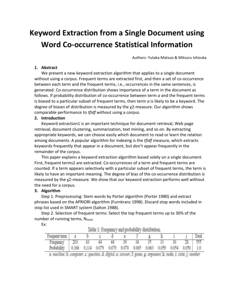
Keyword Extraction from a Single Document using
Word Co-occurrence Statistical Information
Authors: Yutaka Matsuo & Mitsuru Ishizuka
1. Abstract
We present a new keyword extraction algorithm that applies to a single document
without using a corpus. Frequent terms are extracted first, and then a set of co-occurrence
between each term and the frequent terms, i.e., occurrences in the same sentences, is
generated. Co-occurrence distribution shows importance of a term in the document as
follows. If probability distribution of co-occurrence between term a and the frequent terms
is biased to a particular subset of frequent terms, then term a is likely to be a keyword. The
degree of biases of distribution is measured by the χ2-measure. Our algorithm shows
comparable performance to tfidf without using a corpus.
2. Introduction
Keyword extraction1 is an important technique for document retrieval, Web page
retrieval, document clustering, summarization, text mining, and so on. By extracting
appropriate keywords, we can choose easily which document to read or learn the relation
among documents. A popular algorithm for indexing is the tfidf measure, which extracts
keywords frequently that appear in a document, but don’t appear frequently in the
remainder of the corpus.
This paper explains a keyword extraction algorithm based solely on a single document.
First, frequent terms2 are extracted. Co-occurrences of a term and frequent terms are
counted. If a term appears selectively with a particular subset of frequent terms, the term is
likely to have an important meaning. The degree of bias of the co-occurrence distribution is
measured by the χ2-measure. We show that our keyword extraction performs well without
the need for a corpus.
3. Algorithm
Step 1. Preprocessing: Stem words by Porter algorithm (Porter 1980) and extract
phrases based on the APRIORI algorithm (Furnkranz 1998). Discard stop words included in
stop list used in SMART system (Salton 1988).
Step 2. Selection of frequent terms: Select the top frequent terms up to 30% of the
number of running terms, Ntotal.
Ex:
Step 3. Clustering frequent terms: Cluster a pair of terms whose Jensen-Shannon
divergence is above the threshold (0.95x log 2). Cluster a pair of terms whose mutual
information is above the threshold (log(2.0)). The obtained clusters are denoted as C.
Step 4. Calculation of expected probability: Count the number of terms co-occurring
with c ∈ C, denoted as nc, to yield the expected probability pc = nc/Ntotal.
Step 5. Calculation of χ’2value: For each term w, count co-occurrence frequency with c
∈ C, denoted as freq (w, c). Count the total number of terms in the sentences including w,
denoted as nw. Calculate χ’2value following (2).
Pg as (the sum of the total number of terms in sentences where c appears)
divided by (the total number of terms in the document).
nw as the total number of terms in sentences where c appears.
Step 6. Output keywords: Show a given number of terms having the largest χ’2value.
4. Evaluation
Results are shown in Table 7. For each method, precision was around 0.5. However,
coverage using our method exceeds that of tf and KeyGraph and is comparable to that
of tfidf; both tf and tfidf selected terms which appeared frequently in the document
(although tfidf considers frequencies in other documents). On the other hand, our
method can extract keywords even if they do not appear frequently. The frequency
index in the table shows average frequency of the top 15 terms. Terms extracted by tf
appear about 28.6 times, on average, while terms by our method appear only 11.5
times. Therefore, our method can detect “hidden” keywords. We can use χ2 value as a
priority criterion for keywords because precision of the top 10 terms by our method
is 0.52, that of the top 5 is 0.60, while that of the top 2 is as high as 0.72. Though our
method detects keywords consisting of two or more words well, it is still nearly
comparable to tfidf if we discard such phrases, as shown in Table 8.
Computational time of our method is shown in Figure 3. The system is
implemented in C++ on a Linux OS, Celeron 333MHz CPU machine. Computational time
increases approximately linearly with respect to the number of terms; the process
completes itself in a few seconds if the given number of terms is less than 20,000.