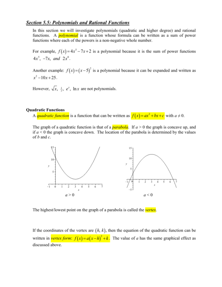
Section 5.5: Polynomials and Rational Functions
In this section we will investigate polynomials (quadratic and higher degree) and rational
functions. A polynomial is a function whose formula can be written as a sum of power
functions where each of the powers is a non-negative whole number.
For example, f ( x ) = 4x 5 - 7x + 2 is a polynomial because it is the sum of power functions
4x 5, -7x, and 2x 0 .
Another example: f ( x ) = ( x - 5) is a polynomial because it can be expanded and written as
2
x 2 -10x + 25 .
However,
x, 1x , e x , ln x are not polynomials.
Quadratic Functions
A quadratic function is a function that can be written as f ( x ) = ax 2 + bx + c with a ≠ 0.
The graph of a quadratic function is that of a parabola. If a > 0 the graph is concave up, and
if a < 0 the graph is concave down. The location of the parabola is determined by the values
of b and c.
a>0
a<0
The highest/lowest point on the graph of a parabola is called the vertex.
If the coordinates of the vertex are ( h, k ) , then the equation of the quadratic function can be
written in vertex form: f ( x ) = a ( x - h) + k . The value of a has the same graphical effect as
discussed above.
2
To find the formula of a given parabola with known vertex, plug the coordinates of the vertex
into the vertex form. Then by plugging any other point in for x and y, we can determine the
value of a.
Example 1
Give the equation of the parabolas shown below.
(a)
(b)
If we know the zeros/roots of the quadratic function, z1 and z2, then we can write the equation
of the function in factored form: f ( x ) = a ( x - z1 ) ( x - z2 ) . Plugging in any other point for x
and y, we can determine the value of a.
Example 2
Give the equation of the parabolas shown below.
(a)
(b)
If the scatterplot for a given data set has the appropriate shape (that is, parabolic), then it can
be modeled with a quadratic regression.
Example 3
The table below shows the number N, in thousands, of vehicles parked in the central business
district of a certain city on a typical Friday as a function of the hour of the day.
Time
N
9 AM
6.2
11 AM
7.5
1 PM
7.6
3 PM
6.6
5 PM
3.9
(a) Let x = the number of hours since midnight. Look at a
scatterplot of the data and comment on why a quadratic
regression may be appropriate.
(b) Find a quadratic regression to model this data.
(c) Use function notation to express the number of vehicles
parked on a typical Friday at 2 PM.
(d) At what time of day is the number of vehicles parked the
greatest.
Polynomials of Higher Degree
A polynomial is a function that can be written as f ( x ) = a0 + a1 x + a2 x 2 +... + an x n where
each ai is any real number.
•
The largest exponent having nonzero coefficient is the degree of the polynomial.
•
Linear functions are degree 1 polynomials
•
Quadratic functions are degree 2 polynomials
Basic Graphs
Degree 3:
Or
1 inflection point only
Degree 4:
Or
2 inflection points possible
Degree 5:
Or
3 inflection points possible
In general, the larger the degree, the more inflection points are possible.
Zeros Determine the Graph
• If z is a zero/root of a polynomial, then ( x - z) is a factor of the formula
•
•
If the graph “bounces” off the x-axis at z, then ( x - z) is the factor
2
Given zeros z1, z2, z3…, we can write the formula in its factored form as:
f ( x ) = a ( x - z1 ) ( x - z2 ) ( x - z3 )...
•
Plugging in any other point for x and y, we can determine the value of a
Example 4
Find the formula for each polynomial shown below.
(a)
(b)
Polynomial Regressions
The TI calculator can find both cubic (degree 3) and quartic (degree 4) polynomials.
If a scatter plot of data has the appropriate shape, such models would be appropriate.
Example 5
The table below gives the average ATM surcharge C, in dollars, in various years.
Year
C
1998
0.89
2000
1.34
2002
1.38
2004
1.39
2006
1.64
(a) Let x represent the number of years since 2000. Look
at a scatterplot of the data and discuss why a cubic
model may be appropriate.
(b) Find a cubic regression model for the data.
(c) Use function notation to represent the average ATM
surcharge, according to the model, in 2005.
(d) Use function notation to represent the average ATM
surcharge, according to the model, in 2013. Why
should we not necessarily trust this prediction?
Rational Functions
A rational function is a function of the form f ( x ) =
polynomials.
p ( x)
where both p and q are
q ( x)
If q ( z ) = 0 but p ( z ) ¹ 0, then the rational function f is not defined at x = z, and the rational
function f has a pole at x = z. The graph of f then has a vertical asymptote at x = z.
If p ( z ) = 0 but q ( z ) ¹ 0, then the rational function f has a zero/root at x = z.
For Example:
1
has a pole at x = 2 and no roots
f ( x) =
x-2
f ( x) =
2x
2x
has poles at x = 3 and x = -2 and has a root at x = 0
=
x - x - 6 ( x - 3) ( x + 2)
2
f ( x) =
f ( x) =
x-2
( x +1)
2
has a pole at x = -1 and a zero at x = 2
4x 2
has no poles and a zero at x = 0
x 2 +1
Limiting Value & Horizontal Asymptote
Recall, as x grows without bound (in the positive or negative direction), the behavior of y
is called the limiting behavior of the function. In the case of a rational function, this is
often a horizontal asymptote – the y-values level off at some specific value.
Look at the graphs above and discuss the limiting value, that is, horizontal asymptote, of
each one.
For rational functions, we can tell just from the formula what the horizontal asymptote
will be or if it does not have one.
Consider f ( x ) =
p ( x)
where p and q are polynomials.
q ( x)
1. If degree of p < degree of q, then y = 0 is the horizontal asymptote.
2. If degree of p > degree of q, then there is no horizontal asymptote.
3. If degree of p = degree of q, then the ratio of the leading coefficients is
the horizontal asymptote.
Example 6
Find the poles, zeros, and horizontal asymptote of each of the following funcitons.
3x 2 + 5
(a) f ( x ) = 2
4x -100
(b) f ( x ) =
x+4
x - 9x +18
(c) f ( x ) =
x 2 + 4x - 21
x -8
(d) f ( x ) =
7x + 4
3x - 2
2