CS664 3/14/2000
Epipolar Geometry and Introduction to Probability and Statistics
Adminstrative Issues:
Anandan guest lecture
Kyros guest lecture
4/3/2000
4/25/2000
PS 1.b due midnight tonight
Oral paper and project abstract due 4/11/2000
No more than 1 page, references to papers, and proposed research project
Camera Geometry:


2 arbitrary cameras at 2 arbitrary points
verged cameras – stereo problem
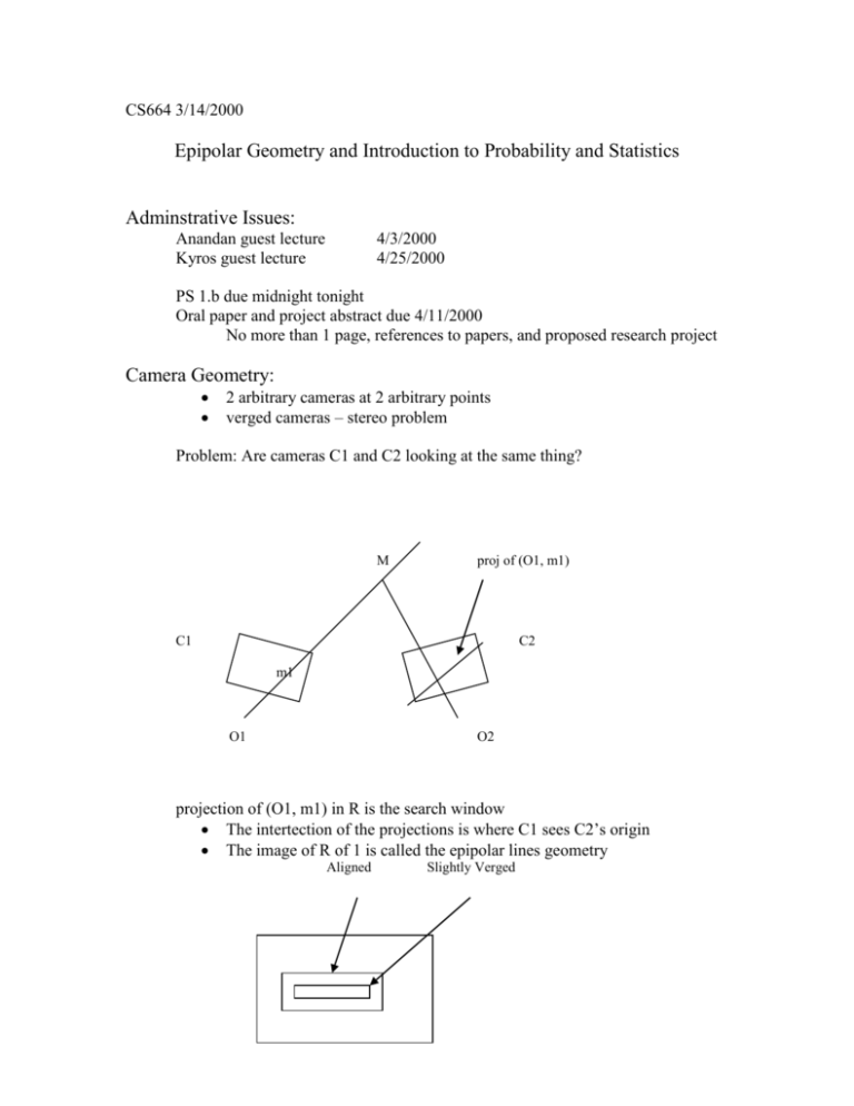
Problem: Are cameras C1 and C2 looking at the same thing?
M
proj of (O1, m1)
C1
C2
m1
O1
O2
projection of (O1, m1) in R is the search window
 The intertection of the projections is where C1 sees C2’s origin
 The image of R of 1 is called the epipolar lines geometry
Aligned
Slightly Verged
For aligned cameras the epipolar lines (your search window) are scan lines.
For slightly verged cameras, use a slightly larger search window.
Estimating Using Epipolar Geometry:


Use sparse methods – find edges/corners to determine the geometry
Use Least Median Squares to tolerate outliers
Calibration of Cameras
 Extrinsic and intrinsic parameters
Extrinsic – 6 degrees of freedom, necessary to estimate this
Intrinsic – foal length f, sampling of LCD grid
-usually fixed
-foal length can change
 Computing the parameters:
Essential Matrix - solves extrinsic parameters
Fundamental Matrix – solves both extrinsic and intrinsic
Self Calibration – difficult to use in a real scene, but works well in
controlled experiments
Structure from Motion – Faugeras ‘93
Probability and Statistics
Min E(f) is a statistical estimation problem.
Probablility
Possible outcomes S – samples, elements, events ()
S is a partition of the universe (all possible outcomes) as fine as we wish
to make it.
Event Space F subsets of  closed under:
F  , 
Complement: A  F, then Ā F
Countable Unions
Discrete Space has size 2||
F is called a σ – field if it has the above properties.
Events
Events are Venn Diagrams, and have the laws:
AB = A∩B
A+B = AUB
A+B = B+A
A(B+C) = AB+AC
Example: Imagine you flip two coins.
Possible Outcomes are HH, TH, HT, TT
F = {, , {HH, HT}, {TH, TT}}
P:F → [0,1]
P() = 0
P() = 1
P(AUB) = P(A) +P(B) – P(A∩B)
Probability space is (, F, P)
Conditional Probability
Given P(A) ≠ 0
P(B|A) = P(A∩B)/P(A)
Venn Diagram
A∩B
B
A
P(B) = P(B|A)P(A) + P(B| Ā)P(Ā)
Given that Ai, i = 1..n are the partitions of , P(B) = Σi P(B|Ai)
A, B are independent if and only if P(A∩B) = P(A)P(B)
Random Variables
Intuitively RV is X:  → Z or R
Distribution Function
X:  → R under the assumption {ω:X(ω) ≤α}F for all α
We can measure the probability of an RV ≤α
If F = 2|| then {ω:X(ω) =α}F for X discrete
P({ω:X(ω) ≤α}F) is written as P(X= α)
event
α
6
8
10
P(X= α) as a function of α is called PMF – probability mass function
The PMF is essentially a histogram
α
6
8
10
P(X≤ α) as a function of α is called CDF – cumulative distribution
function – is monotonically non-decreasing function of α that has the
Properties:
F(-∞) = 0
F(∞) = 1
1
α
PDF – Probability Density Function f(α) = d/dxF(α)
1
α
Note: PDF does not equal PMF, f(α) is not the chance of X= α
Expectance
For RV X(discrete), E[X] = Σ α αf(α) ie the weighted sum
For some g(X)
E[g(X)] = Σ α g(α)f(α)
If g(X) = Xn then E[g(X)] is the nth moment
If g(X) = (X-E[X])n then E[g(X)] is the nth control moment
1st moment = E[X] mean
2nd moment = σ2